How to Create Year and School Calendar with Dynamic Date Markers
As you may know, I provide free and paid calendar templates that you can download every year. All of them have dynamic date marker where specific dates in calendar will be marked with variety colors based on specific color rules. In year calendar models, you can see event tables where each tables has different color rules, either they are single dates or consecutive dates tables. If you put event date in single date tables, respective single date will be marked with color specified by color rule applied for that table. If you put event dates in consecutive date tables, you will see particular dates in the calendar, start from date you put in start date column and end from date you put in end date column, turn to particular colors.
You can’t see the formulas in my free calendars because they are protected. But, I will show you how to create it if you didn’t plan to purchase the paid version and want to create it by yourself.
1. CREATE YEAR CALENDAR
In this tutorial, I will create a calendar for year 2016. I use a simple approach to create the calendar since I will focus on showing you how to create conditional formatting rule to change date colors. I created the calendar by putting the start date of all months in year 2016 on correct weekday name cell. Then, continue filling remaining cells by creating formula to add the dates automatically and stop the addition if it reach the end of the month.
Here is step-by-step instruction to create the basic calendar. I will start from the January table.
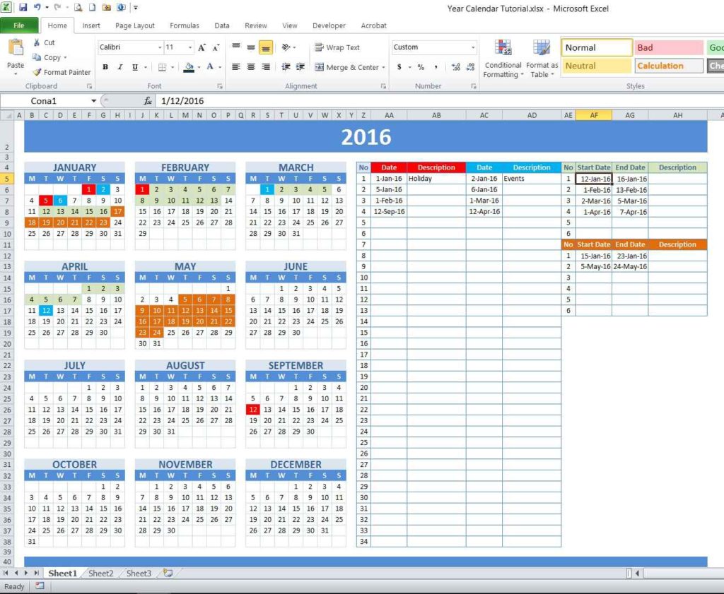
Create 8 rows x 7 columns. Since this is excel, you don’t need to insert anything like Word :). This is the area where you will work in the beginning
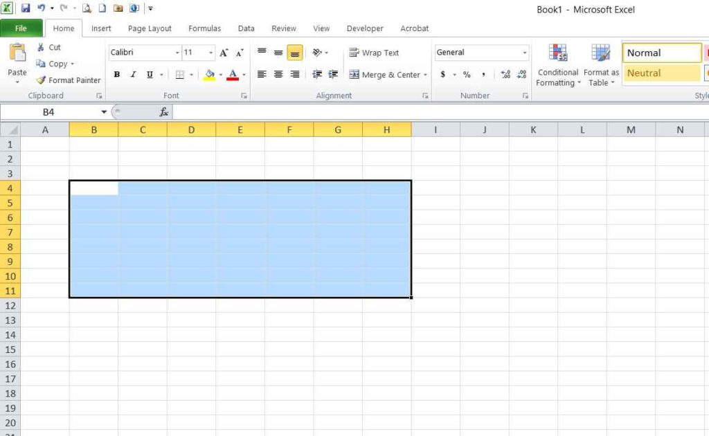
Merge the first row and write the name of the month
Write initial of each day name in the second row
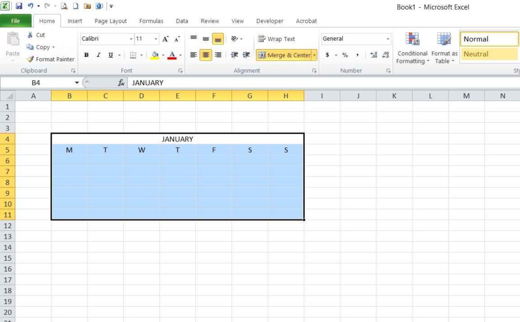
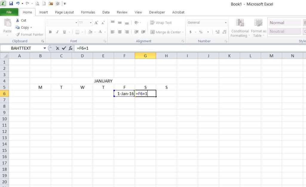
Tag the day of the first day and put in correct cell. In this sample, 1st January falls on Friday.
Use this simple addition function to add dates in sequence in next cells automatically.
- Put F6+1 in cell G6 and drag G6 cell until H column.
- Put H6+1 in cell B7
- Put B7+1 in cell C7 and drag C7 cell until H column
- Select B7:H7 cell, and copy them
- Paste it in cell B8:H9
Create a formula to stop adding dates when it reaches the end of the month. Or, you can just stop it manually.
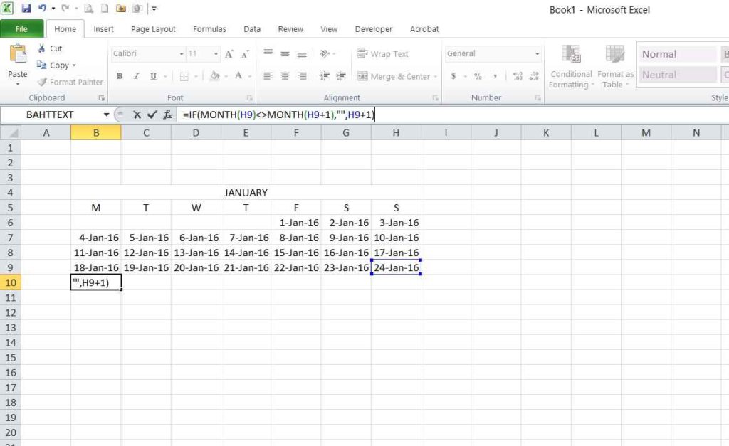
Formula in cell B10
=IF(MONTH(H9)<>MONTH(H9+1),””,H9+1)
This formula basically checks whether the month of date in cell H9 is similar with the month of date if the date in cell H9 is added by one. If the condition is met, than the date addition is continued, if it isn’t then it is stopped.
Create similar formula with different cell reference in cell C10
Formula in cell C10
=IF(B10<>””,IF(OR(B10=””,MONTH(B10)<>MONTH(B10+1)),””,B10+1),””)
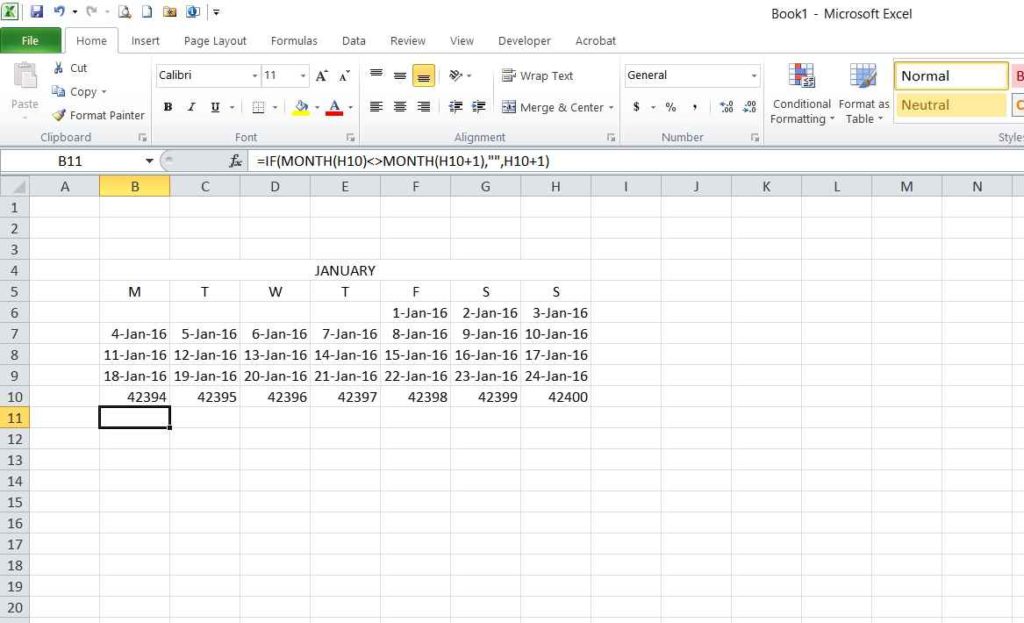
- Copy and paste this C10 formula to cell D10:H10.
- Copy and paste cell B10:H10 to cell B11:H11
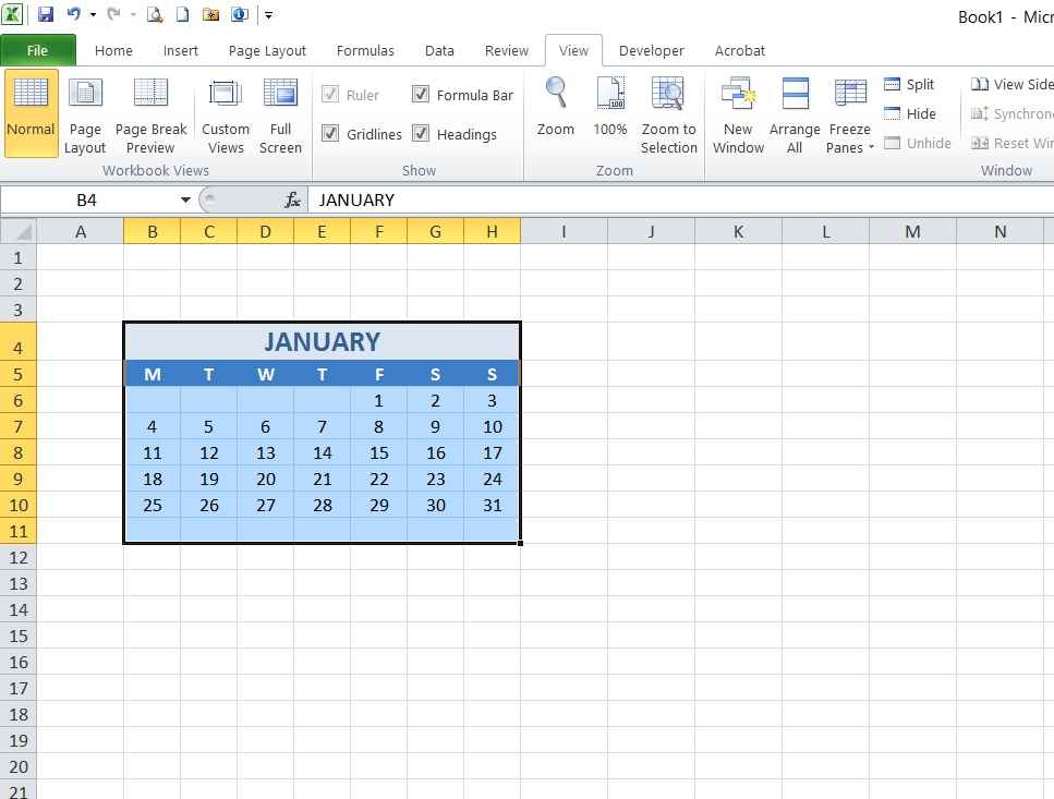
You have completed all formulas in the first month table. But, as you can see in picture below, it is still as it is. It needs to be tidied up.
Personalizing the table (formatting the dates, colorizing its header and align its column width). Change all dates format to show only day number by selecting cell B6:H11 and go to Format Cell menu (you can right click on that selection and select format cell). Go to Number tab menu > Custom. Then type “d” as number format code in its input bar. “d” is the initial of Day in English. It could be other initial in other language.
After you finished with this table, you can copy this table and paste it next to it for creating the second month, February.
As shown in picture above, after you finished duplicating January month table for the second table, you can start customizing pasted table by :
- Changing month name from January to February
- Putting the first date of February in correct weekday cell, and tidy up the first row of month February. Formulas below the first row (row 7 to 11) will be adjusted accordingly.
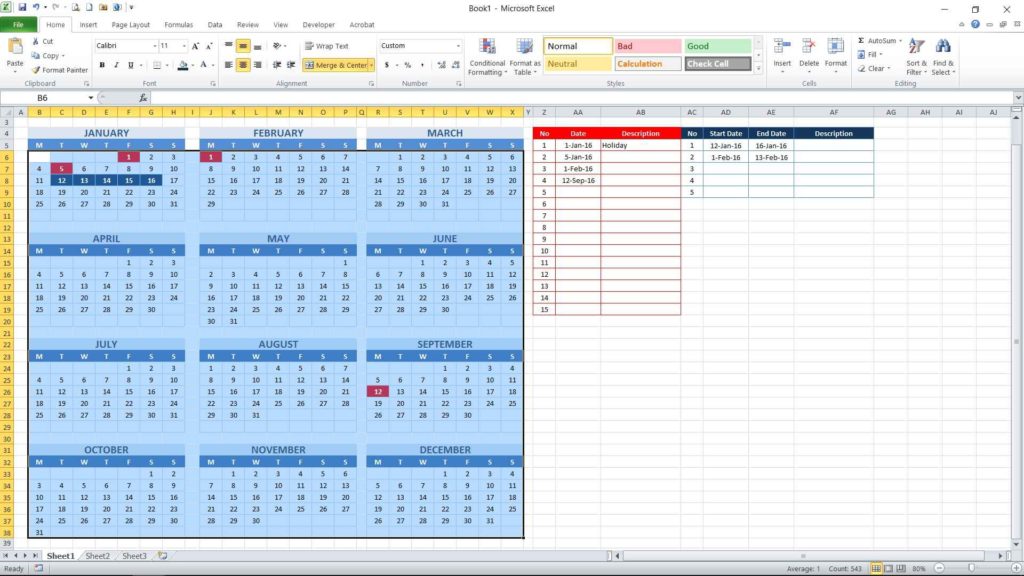
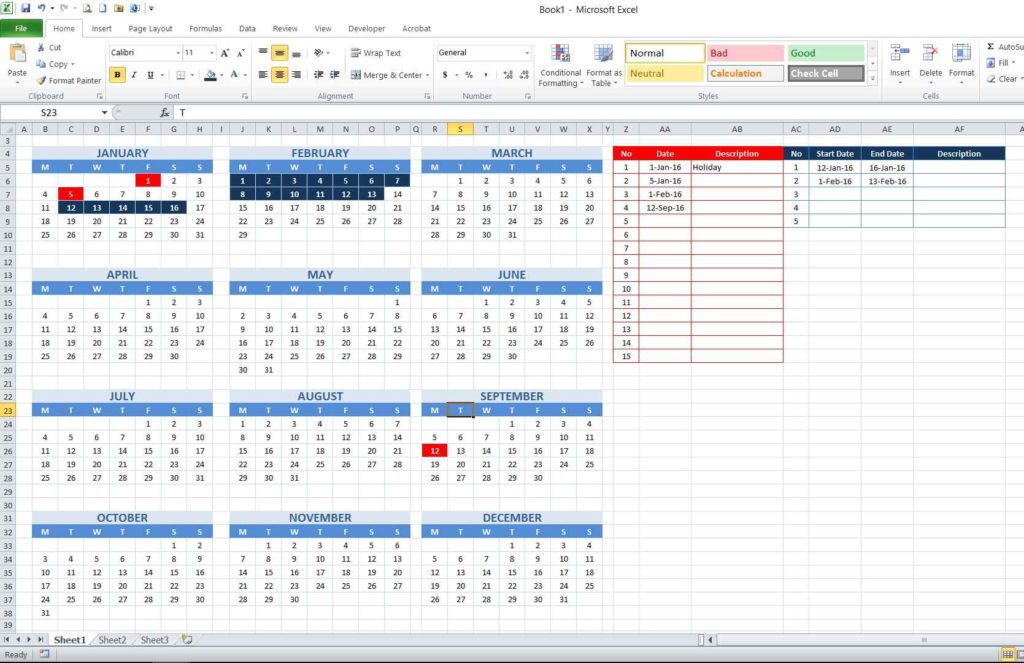
- Repeat all steps above until all 12 months are created. Final year calendar will look like picture below.
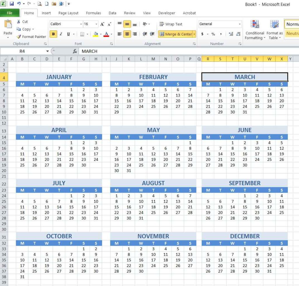
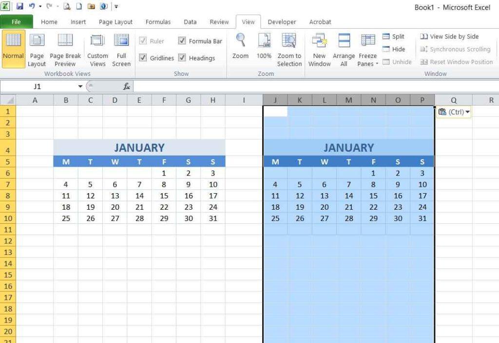
Notes : I select and copy column B:D and paste it into column J:P for duplicating month January format to month February. You can do similar steps for March as well. But, you must select row 4:11 or select specific month for remaining months.
2. CREATE SINGLE DATE EVENT TABLE AND CONDITIONAL FORMATTING RULE
This is the main focus of this tutorial. You can read it carefully to fully understand how to map dates into correct conditional formatting rules.
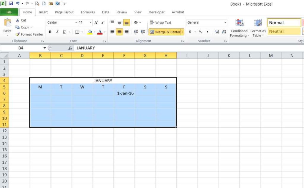
Allocate date rows for events. I allocated 15 rows for events. It means, you can write until 15 events to have it marked in calendars with colors that you have specified. Pay attention to Date column since this column is the main reference of conditional formatting rule.
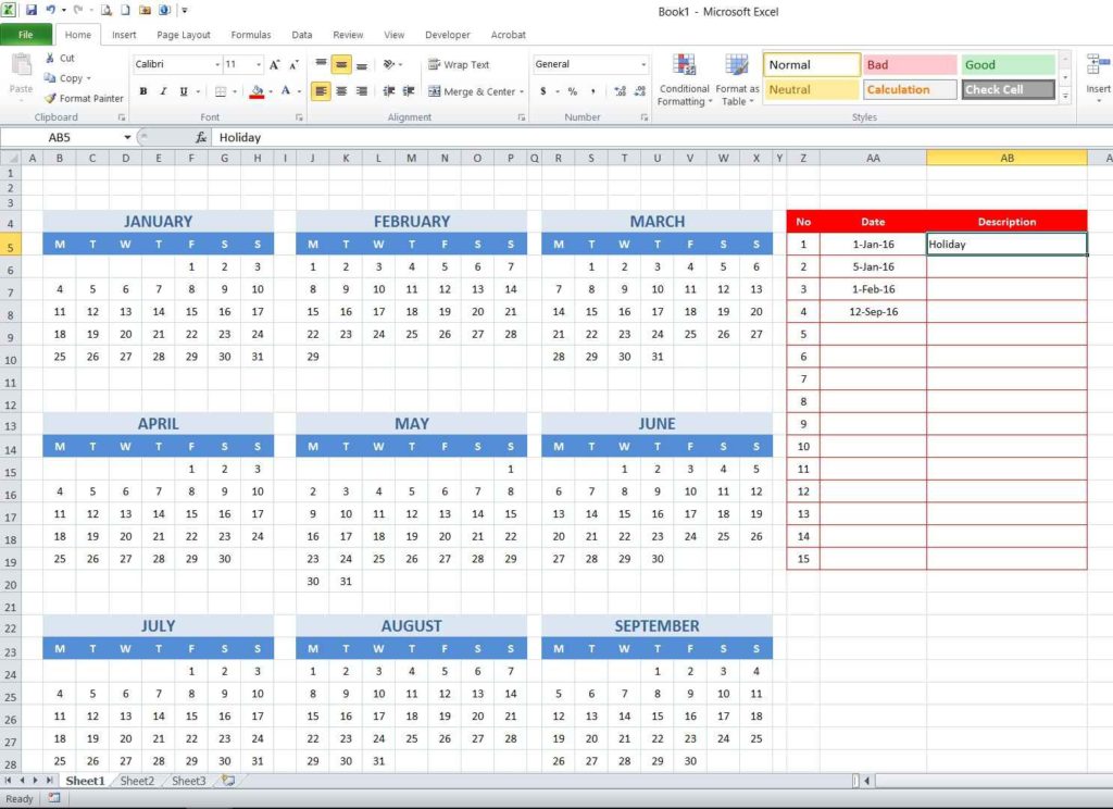
Assign specific name for date group. To make it easier to be used, instead of putting cell $AA$5:$AA$19 as group of event dates reference, you could specify a name for them to make you easier when inserted that group in formula reference. Select this group and type name in name range box at the top left side below menu ribbon as pointed in pictures below. I assigned “Holiday” as its name range.
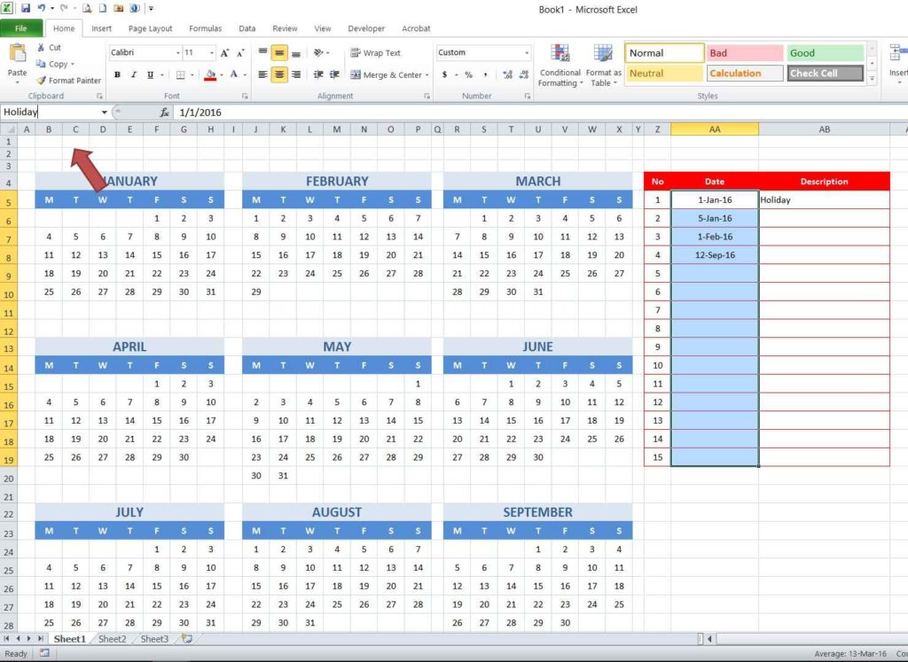
Notes : You can modify this name range (expand or reduce cell reference) in name manager menu. You can access it from Formulas tab ribbon > Name Manager.
Set conditional formatting rule for the calendar. Select all 12 months and then go to Conditional Formatting Tab Menu > New Rule
The logic to map the formula is, if the date in the calendar is similar to date in the event group table, then change its color to specific color.
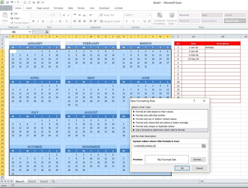
the formula I chose to use to map this logic is
=match(B6,Holiday,0)
Notes:
- Why B6? B6 is the first cell in calendar group selection. It could be any cell references, depends on your own calendar tables and group selection.
- Don’t put Dollar sign ($) in B6. By default, excel will put this dollar sign automatically when you point your mouse to that cell reference. You need to remove it. $ will make the rule works based on cell B6 condition only while removing the sign will make it apply to all cells in your date selection. You can try to experiment with that sign to get a better understanding about its behavior.
Then you can go to format menu to assign specific format if the stated condition is met. Here, I set cells to be filled with red and font color to be changed to white.
You can apply this rule by clicking Apply or clicking OK and closing the conditional formatting rules menu. You can see the result in picture below.
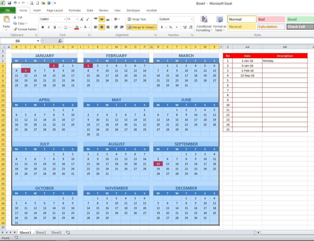
You can start to create the second table for other color by repeating steps above.
You can create as many tables as you want. Remember that one table, or one name range to be exact, can only be assigned with one color.
3. CREATE CONSECUTIVE DATE EVENT TABLE AND CONDITIONAL FORMATTING RULE
This rule is a little bit tricky. It is not as simple as creating formula for single date event table. Here, you need to assign a name range for ONE CELL only. Why? It is only one cell and it doesn’t have to be named. Yes, but you will get confused if you don’t name it when you write a conditional formatting rule for those dates.
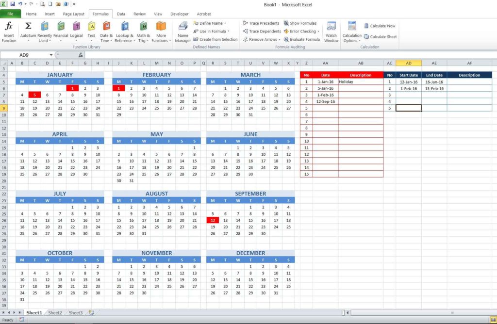
Create Consecutive Date event table.
It needs two columns, one for start dates and other for end dates. In this tutorial, I allocated five rows for this purposes. I set cell AD5:AD9 for start dates column and AE5:AE9 for end dates column.
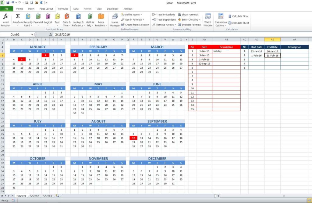
Select and assign names to all start and end dates cells. Set it in similar bar where you put Holiday name for group of single dates.
- 1st row start date, cell AD5 = Cona1
- 1st row end date, cell AE5 = Cona2
- 2nd row start date, cell AD6 = Conb1
- 2nd row end date, cell AE6 = Conb2
Do this until you have 10 names for those 10 cells. It can be any names, you can type names that you can remember easily when you have to work with this cell references.
Set conditional formatting rule. Select all 12 months again and then go to Conditional Formatting Menu > New Rule
The logic is to check whether the calendar date is between specific start and end dates as typed in consecutive event date table. We are not using MATCH function here. I use a simple OR and AND condition for this logic implementation. Is it simple? Yes, if you only have several consecutive dates. But, you will write a very long formula if you want to have more tables and more periods.
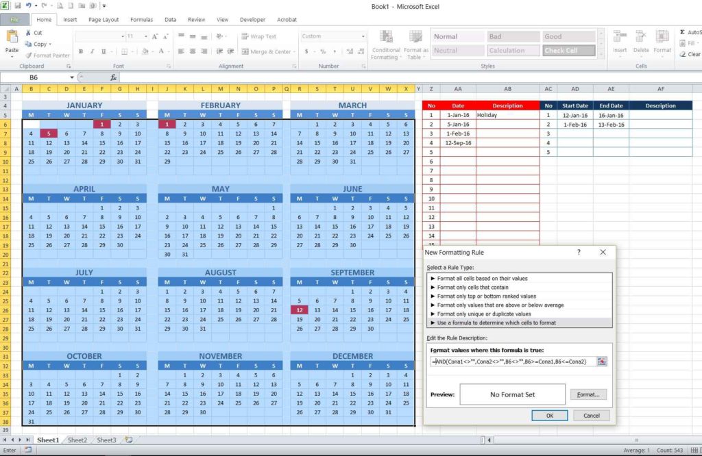
The formula to check the date with the first period is
=AND(Cona1<>””,Cona2<>””,B6<>””,B6>=Cona1,B6<=Cona2)
Remember : Cona1 is the start date and Cona2 is the end date of the first event period
It will check whether the cells are empty or filled (Cona1<>””,Cona2<>””) and it will check whether the calendar date (B6) is within the specified period (B6>=Cona1,B6<=Cona2). I set dark blue color to fill respective dates if the condition is met and change the font color into white.
You can check the result by clicking Apply. If it works as expected, you can start creating the formula for the second row of the event. It should be typed :
=AND(Conb1<>””,Conb2<>””,B6<>””,B6>=Conb1,B6<=Conb2)
You can type it in your Notepad, or blank area of your worksheet before combining them in conditional formatting rules window.
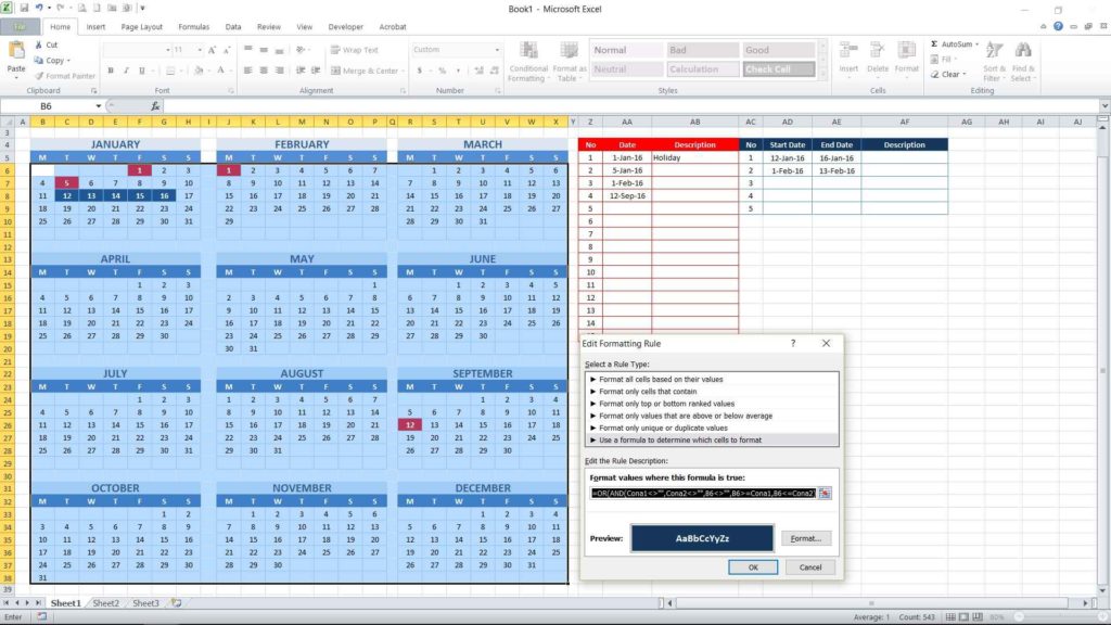
Based on two formulas above, you have 2 conditions that will have similar colors when the condition is met. To combine those, you can use OR function, and the format will be like this (combine this in notepad and then copy and paste it into rule window):
=OR(AND(Cona1<>””,Cona2<>””,B6<>””,B6>=Cona1,B6<=Cona2),
AND(Conb1<>””,Conb2<>””,B6<>””,B6>=Conb1,B6<=Conb2))
Check again whether your formula is typed well.
You can continue completing the formula for all event periods. The final formula should look like this :
=OR(AND(Cona1<>””,Cona2<>””,B6<>””,B6>=Cona1,B6<=Cona2),
AND(Conb1<>””,Conb2<>””,B6<>””,B6>=Conb1,B6<=Conb2),
AND(Conc1<>””,Conc2<>””,B6<>””,B6>=Conc1,B6<=Conc2),
AND(Cond1<>””,Cond2<>””,B6<>””,B6>=Cond1,B6<=Cond2),
AND(Cone1<>””,Cone2<>””,B6<>””,B6>=Cone1,B6<=Cone2))
Now you see how long the formula is. It is for five event date period. You will have a very long formula that needs to be typed carefully if you want to cover more periods.
That’s all guys. You can start personalizing the calendar and experimenting with those formulas. You can follow similar steps to create School calendar which usually doesn’t start from January. If you want to use ready-made year calendars you can get it in 2016/2017 School Calendar and 2017 Calendar posts (formulas in free versions are protected though). If you already have the paid version or plan to purchase one so you don’t have to start from the scratch, you can apply above method to customize it. But, newest 2017 calendar models have different conditional formatting rules where it uses additional function to accommodate typing single and consecutive dates in similar table.
There are video tutorials that you can watch in youtube as well.
Hi Dann,
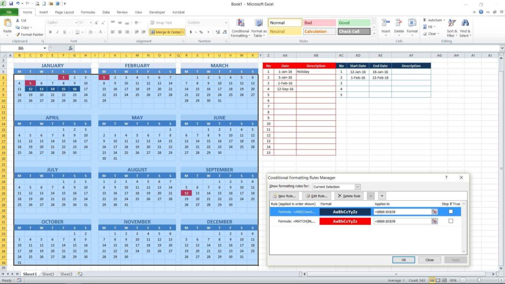
The order of conditional formatting rule will determine the modification that will be applied to particular cell if value on that cell is fit with more than one condition.
Regards,
Ignore second comment .. figured it out by watching the video. I needed to move the holiday formula above the ‘con’ formula. That step isn’t mentioned in either the video or this page, but looking closely at the video I saw you do that.
I’ve followed your steps and have it working almost as expected. However, once I apply the consecutive dates the holiday dates background colour disappears and they become the the background colour of the consecutive dates, if you know what I mean. It’s like the ‘con’ colour is over-writing the ‘holiday’ colour. How do I make sure a holiday that falls within the ‘con’ range is still coloured as a holiday??
Can this be turned into a perpetual calendar?
Hi,
Very good instruction. Do you have tutorial to create this calendar but for multiple events on the same date?
First of all, thank you so much for the tutorial! This has been extremely helpful! I am having an issue that perhaps you can assist me with. I have events listed that go through Saturday and Sunday but don’t need the weekends highlighted how can I keep those days from being highlighted?
This response is for Farley and anyone else wishing for a multiple event calendar.
For a calendar with multiple events for the same day I have created it when I was creating this calendar, I was already thinking ahead, and wanted the same thing, with four events and four different colors on the same day for my Global Purchasing team at work.
With some patients, you could add as many tables and colors as you want. For my calendar I used the four colors of Lt Green (153,255,153) for “Holiday”, Lt Blue (102, 204, 255) for “Floating Holiday”, Lt Yellow (255, 255, 153) for ‘Vacation”, and Lt Pink (255, 204, 255) for “Birthday”.
Posted it on our Share Point site and all twelve associates can access it when it is convenient for them. I also locked the file, except for the areas I needed the associates to input their dates, also, for simplicity I did not use Musadya’s example to create consecutive date event, I just figured it was simpler for the team to add each date separately, and it works great!
How can I do the “CREATE CONSECUTIVE DATE EVENT TABLE AND CONDITIONAL FORMATTING RULE” in google sheets?
Hello,
Thank you for these resources! I have downloaded the template for 2021 Calendar Model 5 – V2.6 – with Right Notes – Sunday.xlsx and cannot seem to get the year to adjust for 2022 and to duplicate the sheet for 2023 onwards. Is there a place where I can download templates for these updated years? I tried to follow the tutorial, but am not a Google Sheets whiz, so I’ve been struggling.
Thanks for your help!
I am looking for a training Calendar beginning Nov 01, 2022- Dec 25, 2023. I need it to contain 4 hours of training per instructor per week. Sessions are weekday. Instructors are two per week, with a ratio of 12 students per instructor for 24 students total per week. Training will consist of 4 hours am and 4 hours pm. There will be a total of 8 instructors that need to be rotated throughout. This training will be done on a monthly basis.
Please provide a cost if your are still available, and form of payment.
Thanks,
Joe
The formulas in our language EXCEL differs.
So question: Can I download your Excel sheet ??