Create Your Own Soccer League Fixtures and Table
Finally I finished my tutorial on creating sports league standing table using Microsoft Excel, as promised. You can use this tutorial not only for creating soccer or football competition like my sample, but also you can use it for any competitions that follow the same schemes.
Step 1 : Define Participant Teams
At the beginning, you need to define the number of teams that participate in the competition. I define 8 teams as participants in this tutorial
Step 2 : Define Competition or League Type
You have to define the competition type. You will need this to control your fixtures table. Although this one has no direct effects in the formula, it will give you additional concerns when you need additional factor to decide the competition winner, just in case there is a tie position for some teams when all competition matches are completed. For example, if you pick full competition type where each team will meet twice in home and away game, you can make the goal made by away team in away game have more weight than goal in home game as decision factor to rank the team.
Step 3 : Define Competition Rule
You have participants, you already defined the competition type, now, you have to define rules needed to rank the team . And in this tutorial, I use the following rules to define the standing position :
Competition Basic Rules :
- The final rank will be decided after all matches are finished
- A team will get 3 points for winning, 1 point for draw and no points for defeat
Competition Standing Rule :
- One team will be above other teams if it has more points than other teams
- If there are two or more teams have the same points, the higher rank will be decided by better goal differences
- If there are two or more teams have the same points and the same goal differences, the higher rank will be decided by better goals scored for
- If there are two or more teams have the same points, goal differences, and goals scored for, higher rank will be decided by better away goal scored
You can add more rules for the competition to define the ranks, because once you know how to formulate it, any rules can be interpreted into excel formula easily.
Step 4 : Create Blank Dummy League Standing Table Sheet
Create a dummy league standing table worksheet. Why ? Because you need fixed columns for teams to be used as formula references, where all values picked and calculated from fixtures result will have fixed cell places inside the table. By doing that, it will be easier to manage all formula needed to get your team ranking based on any rules you specified. Is it possible to have just one table ? It is possible, but it is more complicated because you have to make one long formula with many conditions within one cell.
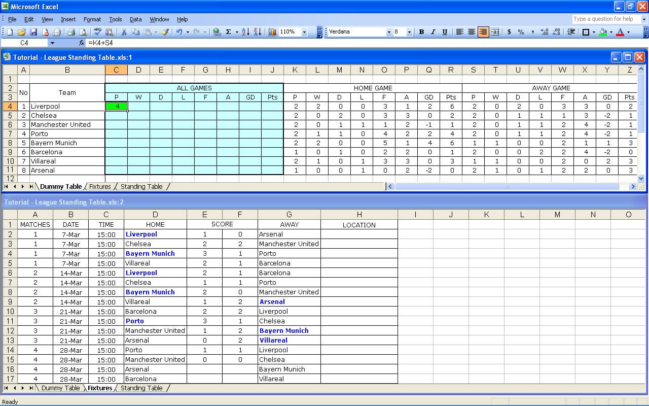
You can see my blank dummy standing sheet below. As I mention above, this is a full competition worksheet with home and away matches.
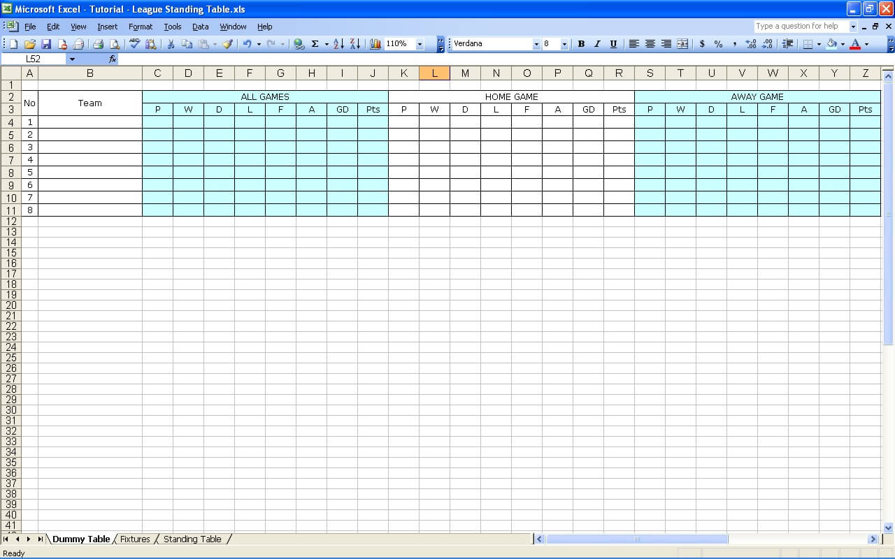
The following abbreviations are common football abbreviations used in league standing tables :
P : Played, W : Win, D : Draw, L : Lose, F : Goal Scored For, A : Goal Scored Against, GD : Goal Difference, Pts : Points
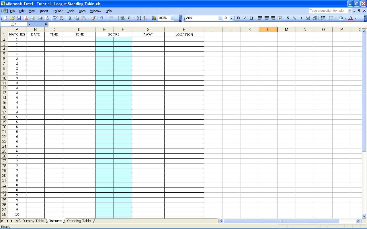
Step 5 : Create Blank Fixtures Worksheet
Now, you have to create blank fixtures worksheet where you can setup your league fixtures and fill the matches result. It is easier to make it in a separate worksheet because you can alter or change the layout later without affecting other table formulas.
One thing you have to keep in mind is, once you defined the column, you should not alter the position of the columns, because it will affect the formula references in other worksheet, except you are not forgetting to change the reference.
There will be 56 matches that will be calculated in the table. The number come from this calculation:
- There will be 4 matches per week or per some period of time,.
- Each team will face 7 other teams twice
And this 56 matches can be interpreted into 56 matches rows in your table.
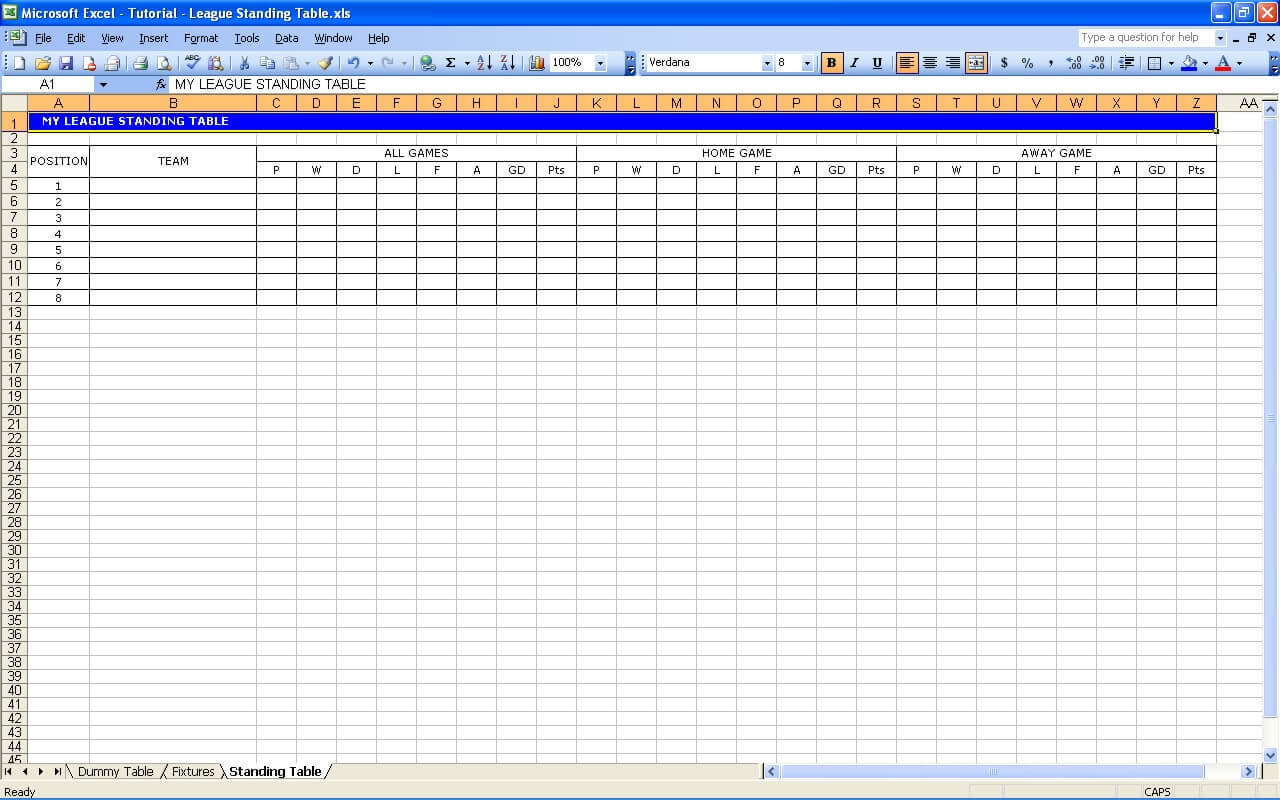
Step 6 : Create Blank Standing Table Sheet
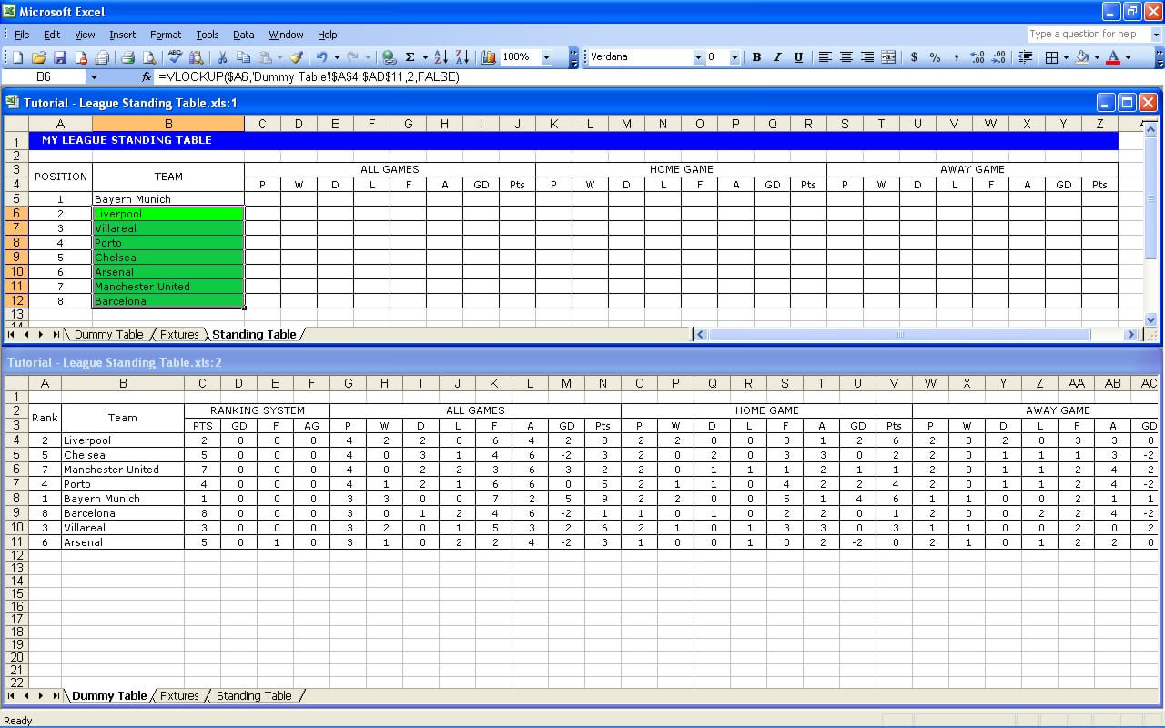
And now, you can create the standing table, with the same structure with Step 4, except for this one you put position number as your fixed reference. Just make the same table and put position number 1 – 8 in column A as seen the picture below.
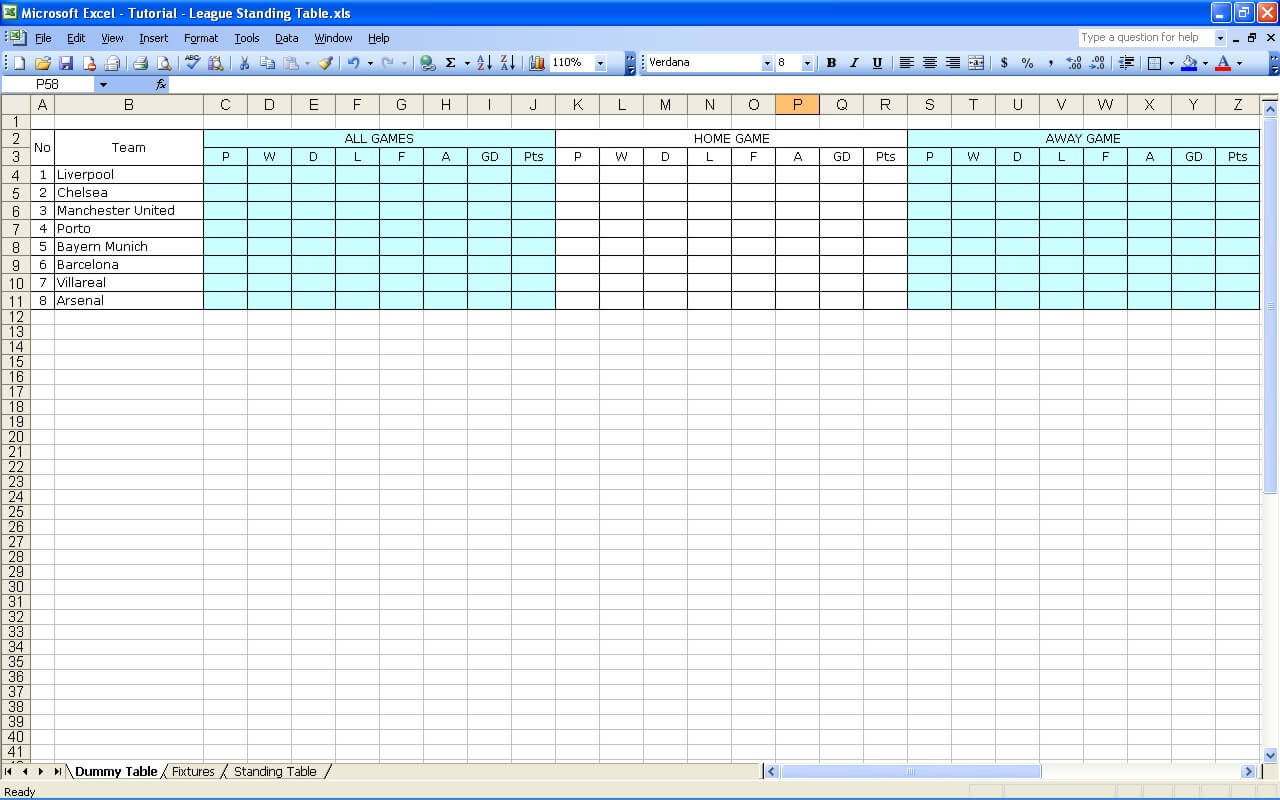
Step 7 : Fill Team’s Name in Dummy League Standing Table Worksheet
All worksheets and basic tables are ready. Before proceeding to prepare the formula needed to automate all the standing process based on competition rules in Step 3, fill your dummy table with your team’s name. My sample worksheet can be seen in picture below.
Step 8 : Fill Dummy Result in Fixtures Worksheet
The reason why you should fill dummy result in fixtures worksheet is to ease your understanding on how the formula will work in dummy table worksheet. You can fill all columns or just some parts of them. In my example, I fill 14 matches with random results.
After finished filling dummy results in fixtures worksheet, go back to dummy table worksheet. Here you will have to create formula to grab all the results in fixtures sheet into the dummy table worksheet.
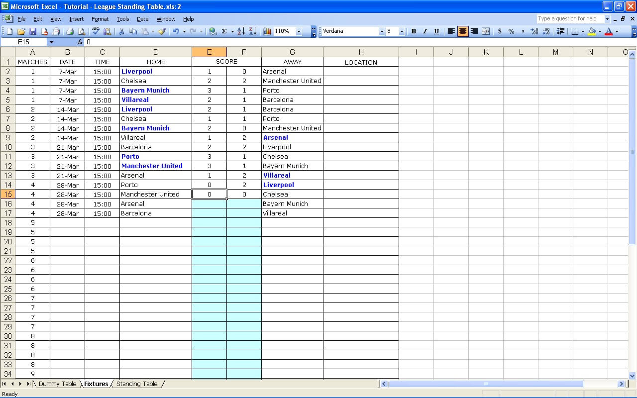
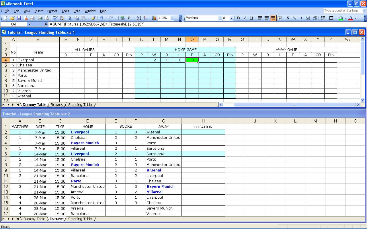
Step 9 : Create Formula for Home Matches Win Results
The first formula I create in dummy table worksheet is formula to grab all home matches results. There is 8 defined columns in fixtures sheet. In this tutorial, we are going to only use four columns, columns D to G. You might need other columns If you plan to expand your league to include analysis, charts or other functions.
Now, I will create formula for Liverpool home matches, the first team in the team column in dummy table worksheet. As you can see in fixtures worksheet, we can summarize Liverpool home matches as follows :
- Liverpool played twice
- Liverpool won twice
- Liverpool scored 3 goals
- Liverpool got scored against 1 goal
Based on that Liverpool home matches summary, we have to find correct logics to interpret these results and find the suitable excel functions to transform them into correct cell values. There are some excel functions with some combination that can be used to interpret them. I have made some experiments of those excel function combination before I decided to use Sumproduct function, which I think this is the shortest one.
You can see the basic structure of sumproduct function below :
Cell Value = sumproduct((ConditionA)*(ConditionB)*(ConditionC)*()…)
If the condition is met, the value will be 1, if the condition is not meet, the value will be 0. If all conditions is met, it means the multiplication of those conditions will be 1. This will work in loop until all set of conditions are verified. And the Cell Value will be the sum of those set values.
If you read the explanation about sumproduct in excel help, probably you won’t get the explanation for this kind of purposes, because excel help just provide you basic information about that function. You can google for this function if you need more explanation.
And the formula for this example to be put in cell L4 using this function is :
L4 value = SUMPRODUCT((Fixtures!$D$2:$D$52=$B4)*(Fixtures!$E$2:$E$52>Fixtures!$F$2:$F$52))
We need only two conditions to get the value.
Condition A = Fixtures!$D$2:$D$52=$B4 is created to find a team named Liverpool in column D
Condition B = Fixtures!$E$2:$E$52>Fixtures!$F$2:$F$52, is created to find cells where the value of column E is bigger than column F which mean where Liverpool win.
The usage of $ sign is to prevent the cell reference change when you copy the formula to other cells.
L4 value = will be the sum of values from multiplication conditions of those two conditions
If you do it correctly, the value should be 2.
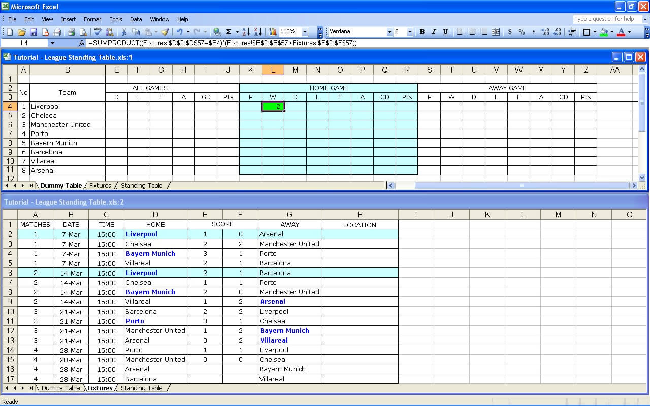
Step 10 : Create Formula for Home Matches Draw Results
Now, move the cell M4 where you have to grab Liverpool draw results in that cell. And like the step 9, there are two conditions that have to be met, but there is one condition that have to be considered, as you can see it here:
M4 value = SUMPRODUCT((Fixtures!$D$2:$D$52=$B4)*(Fixtures!$E$2:$E$52=Fixtures!$F$2:$F$52)*(Fixtures!$E$2:$E$52<>””))
Condition A = Fixtures!$D$2:$D$52=$B4 is created to find a team named Liverpool in column D Condition B = Fixtures!$E$2:$E$52=Fixtures!$F$2:$F$52 is created to find cells where the values are the same, which means draw.
Condition C = Fixtures!E$2:E$52<>”” is created to prevent the Condition B formula take blank cells into calculation. You know, blank cells will be considered as 0 and it will give you draw results. I don’t put a formula for column F because one cell is enough to prevent it.
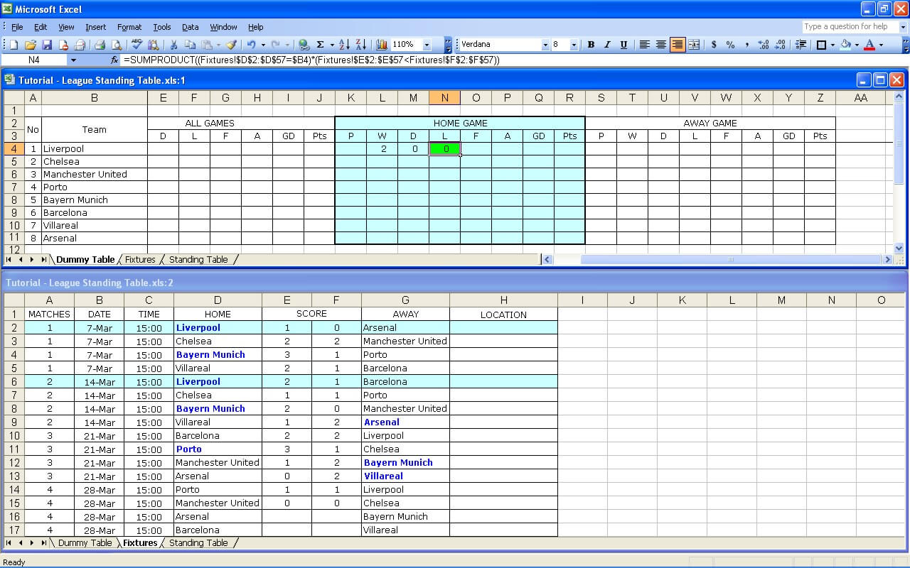
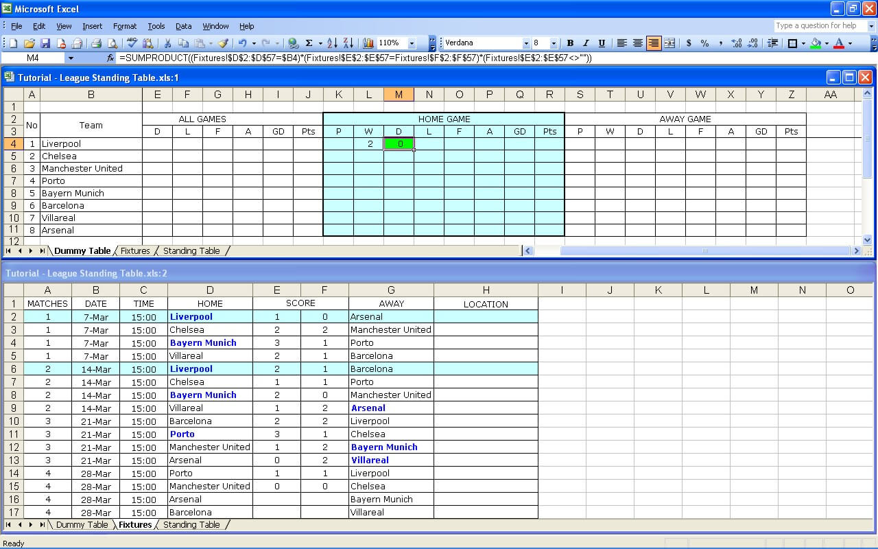
Step 11 : Create Formula for Home Matches Lose Results
After step 9 and 10, I think you know what you have to do in cell N4. You can copy L4 formula and change the logical sign for condition B (see step 9). The complete formula is :
N4 Value = SUMPRODUCT((Fixtures!$D$2:$D$52=$B4)*(Fixtures!$E$2:$E$52<Fixtures!$F$2:$F$52))
You got it right ? Just change the red color sign above and you have completed your formula.
Step 12 : Create Formula for Home Team Goals Scored Results
For this cell, you can skip the sumproduct function. For this one, you use sumif function because you need to add the content of your target columns. So, the formula is :
O4 Value = SUMIF(Fixtures!$D$2:$D$52,$B4,Fixtures!$E$2:$E$52)
Read basic excel help provided in Microsoft Excel if you want to learn more about sumif function.

Step 13 : Create Formula for Home Team Goals Scored Against Results
Copy step 12 formula and paste it into P4 cell. Change the E column reference to F column reference to get the goals scored against value.
P4 Value = SUMIF(Fixtures!$D$2:$D$52,$B4,Fixtures!$F$2:$F$52)


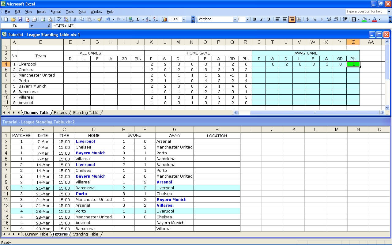
Step 14 : Create Formula for Home Team Points
The value for these cells can be calculated easily. All you have to do just multiply defined points for winning and draw with the number of wins in column L and draws in column M. Except you want to have points also for losing, you don’t have to put value from column N into calculation.
Q4 Value = L4*3+M4*1
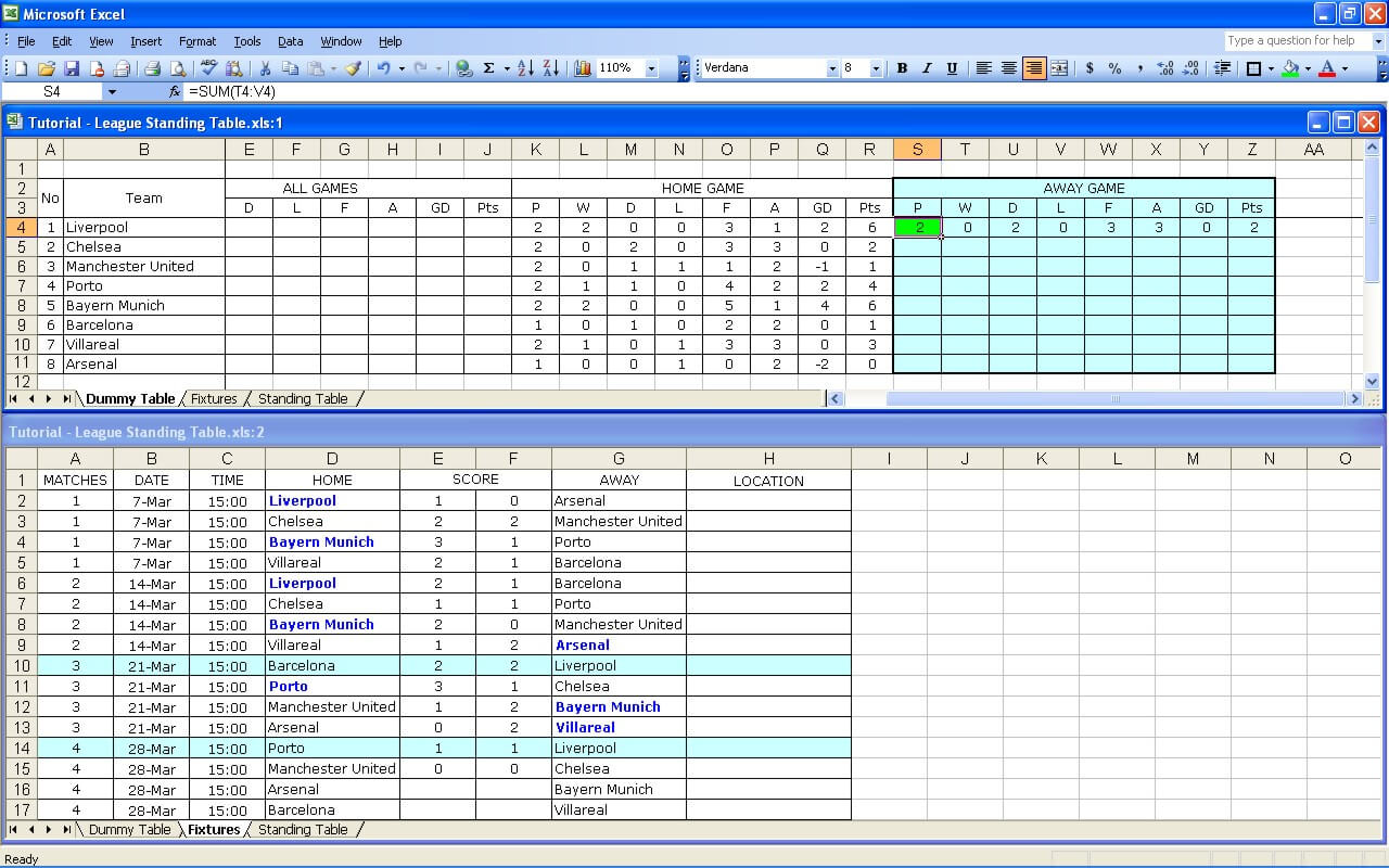
Step 15 : Create Formula for Number of Home Team Played
The value in R4 is basically just the sum of win, draw and lose value in column L4, M4 and N4.
R4 Value = SUM(L4:N4)
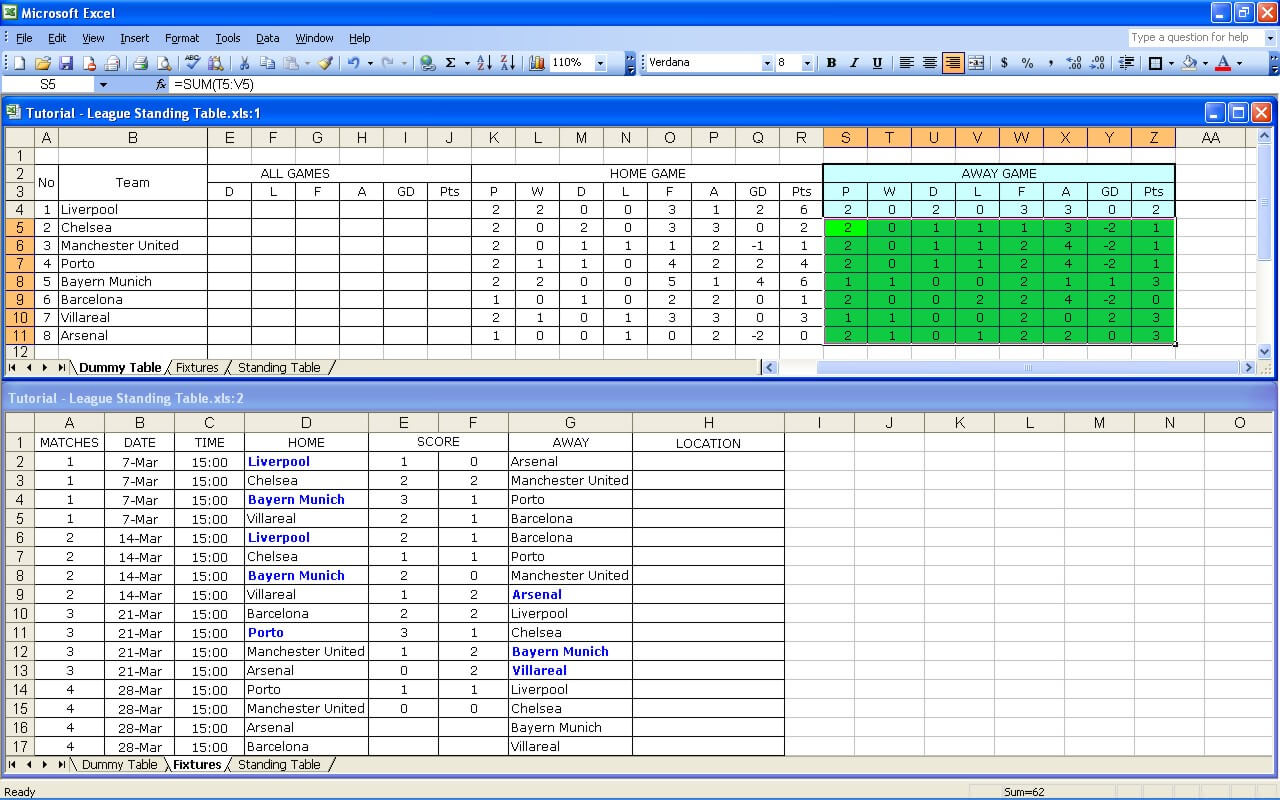
You finished creating formulas for Liverpool Home Matches rows. Check and compare the results with you manual calculation.


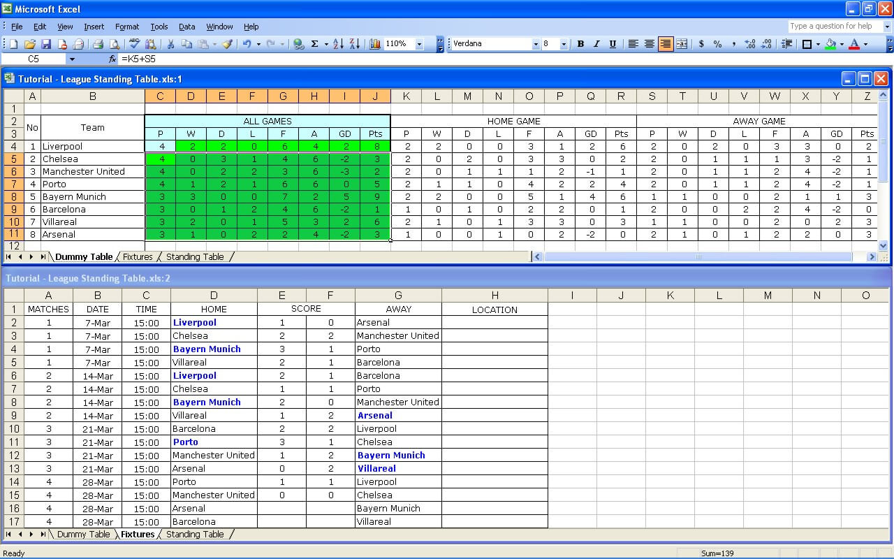
Now, you can simplify the formula for other 7 teams just by copying that Liverpool home matches formula and paste it to 7 rows below as you can see in Picture 14.
Your Home Matches Table is completed now. The next step is creating the formula for Away Matches Table.
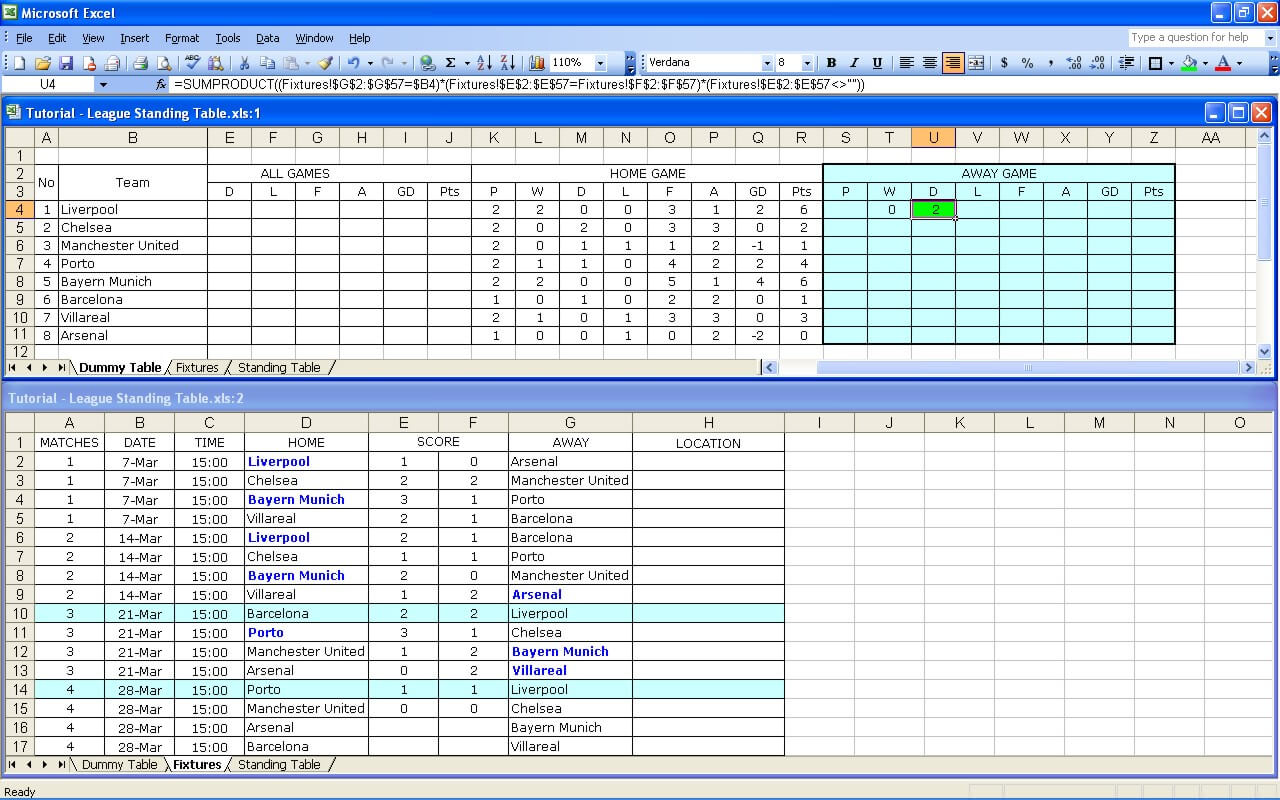
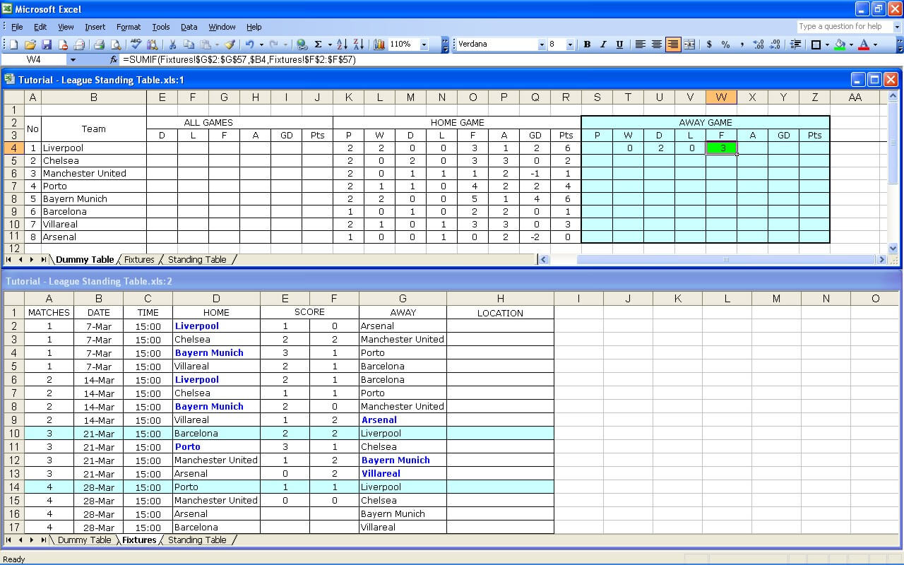
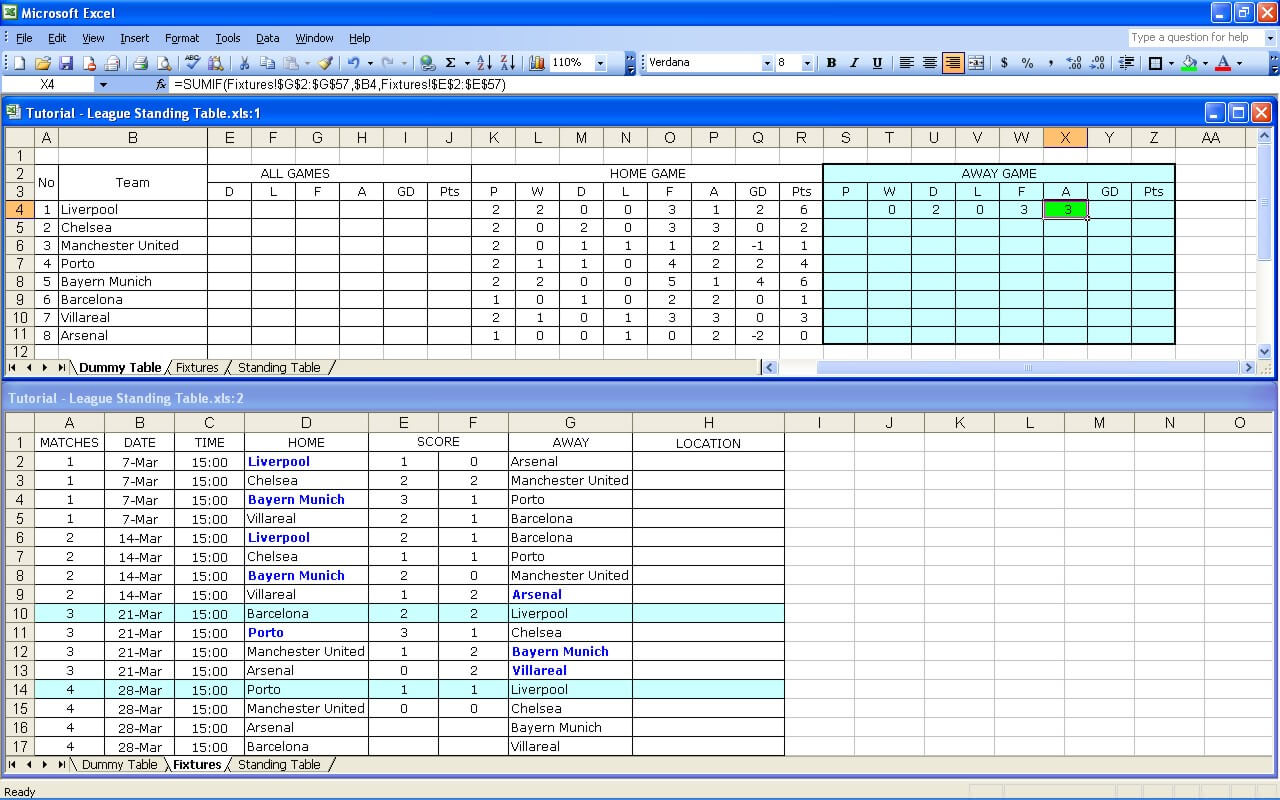
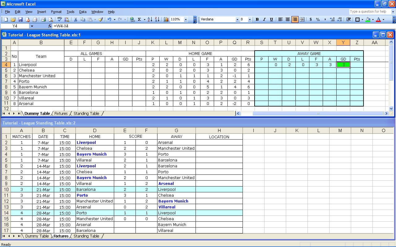
Step 16 : Create Formula for Away Matches Columns
In this table, try to repeat the step 9 – 15. The logic and formula used is the same, except Liverpool is an away team now. So, the Liverpool team will refer to column G in dummy table, goals scored will refer to column F, and goals scored against will refer to column E. I think for this step, you can tryto do it by yourself. I attach the picture 15 – 23 with the formula inside the picture, for you to check your formula.


Step 17 : Create Formula for All Team Matches Results
Because all team matches are sum of all team home and away matches, all you have to do just add corresponding columns to complete the table. And it only needs two steps. First, go to cell C4 and type K4+S4. Copy this cell, select cells C5 – C11, and paste it. You have your table completed now.
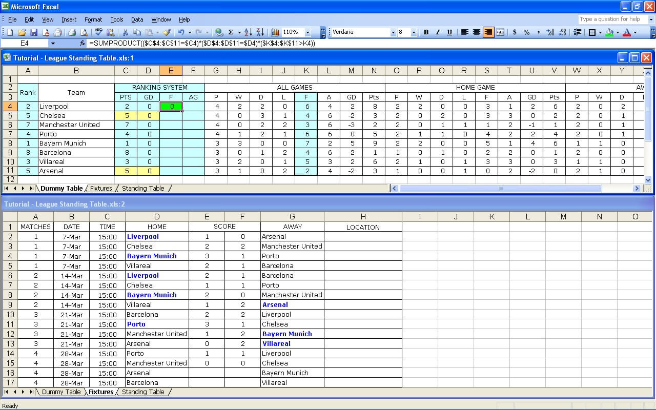
Step 18 : Create Formula for Ranking Position based on Points
And these are the important columns of creating standing table. This is a place where you interpret your competition rules to give you the rank you wanted.
Before go to create formula, you have to insert four new columns between column B and column C. Select column C, right click your mouse and click insert. Do this four times, so you will have blank columns from C to F.
We will interpret the rule one by one. Just to remind you, the first competition rule is
“1. One team will be above other teams if it has more points than other teams”
Go to cell C4 which belongs to Liverpool rank based on points. Manually, you can see that Liverpool is rank number 2 among 8 teams.
Because this is the first condition that have to be met, you can use the rank function provided by excel to get your team rank based on points. So, the formula will be
C4 Value = rank(N4,$N$4:$N11). Copy the formula and paste it to cells C5 to C11 to fill all columns with rank formula.


You can see that the rank function will do basic rank function. And you can see in the example that Chelsea and Arsenal are sharing the same rank, 5, because both are having same points. And you will see that there is no rank no 6. And this is the reason why making league standing table is not as easy as people think.
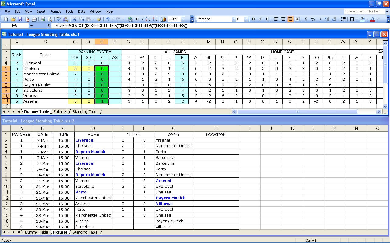
Step 19 : Create Formula for Ranking Position based on Goal Differences
Now, you need to differentiate which team is on top of other. So, we have to interpret rule number two to differentiate them using excel function.
Competition rule number two is :
“2. If there are two or more teams have the same points, the higher rank will be decided by better goal differences”
You cannot use the rank function here because the weight of goal difference for each team is not the same. You have to filter it. So, the most suitable excel function to interpret this is sumproduct function.

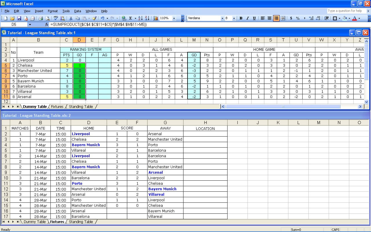
Go to cell D4. The formula we used here is D4 Value = SUMPRODUCT(($C$4:$C$11=$C4)*($M$4:$M$11>M4)).
Condition A = $C$4:$C$11=$C4, is created to find the value in column C which have the same value with C4 value
Condition B = $M$4:$M$11>M4, is created to find value in column M which is bigger than value in M4
D4 Value will be sum of multiplication between condition A and B, just like the formula used in previous steps. Copy D5 and paste it in D4-D11 to get the formula working for other cells.
After you running it, you should see that it will give you the same value for both Chelsea and Arsenal because the GD for both teams are the same as you can see in picture below.

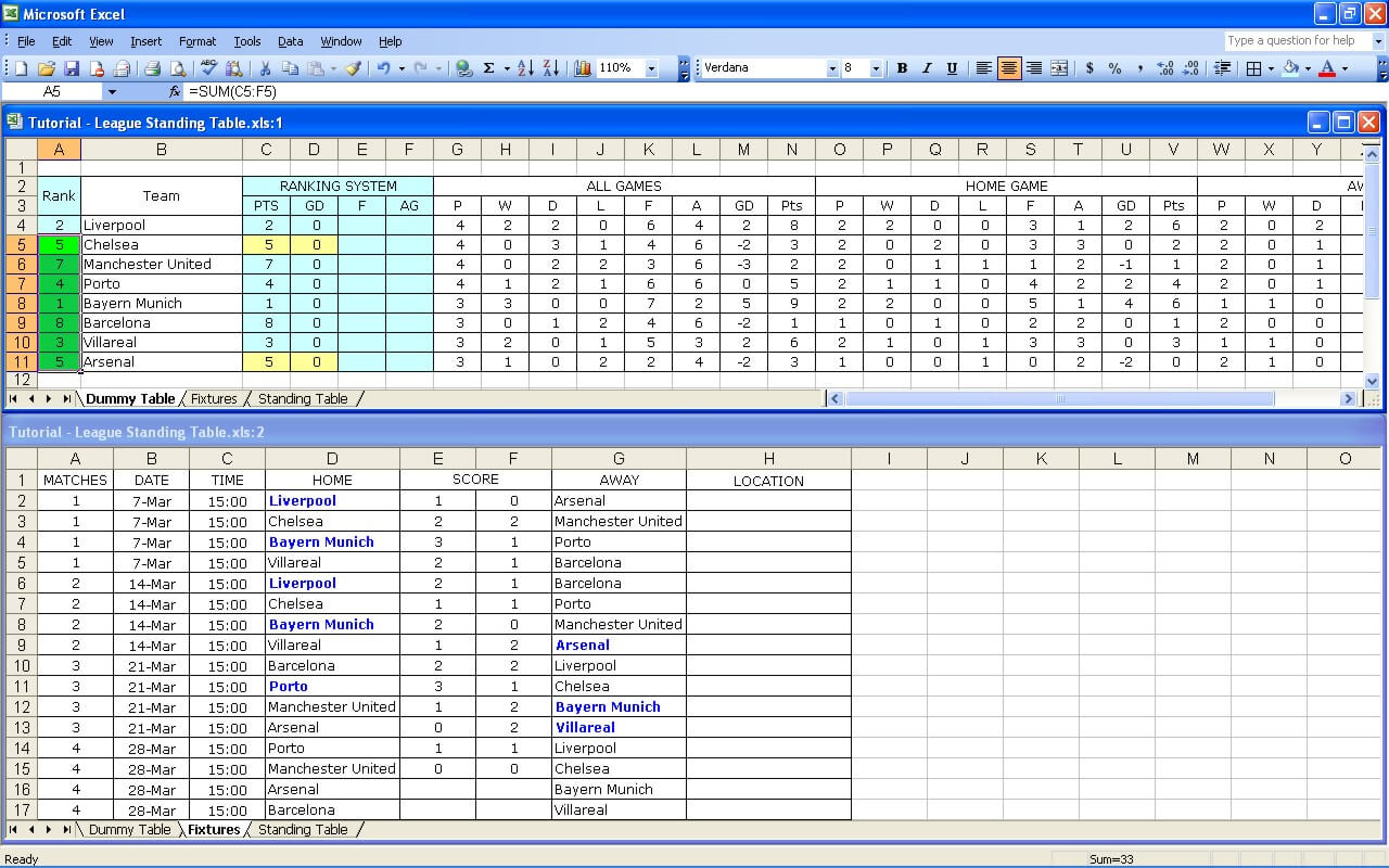
After this step, I hope you understand how the formula worked. And before going to third column or column E, put a formula in column A to sum the ranks of those four columns to get the feeling of the ranking formula you made.
A4 Value = Sum(C4:F4). Copy A4 formula and paste it on column A5-A11. And you have your ranking position that will be used as reference in standing table worksheet. Why it has to be in column A ? Because this column will be used as the first vlookup reference in standing table worksheet, where it can only lookup the right value from the reference.
After running the formula for all teams, you can see that Arsenal and Chelsea still share the same ranking because of their points and goal difference are the same.
Step 20 : Create Formula for Ranking Position based on Goals Scored
So, we need competition rule number three to differentiate their ranking.
“3. If there are two or more teams have the same points and the same goal differences, the higher rank will be decided by better goals scored for”
And this is the function :
E4 Value = SUMPRODUCT(($C$4:$C$11=$C4)*($D$4:$D$11=$D4)*($K$4:$K$11>K4))
Condition A = $C$4:$C$11=$C4, is created to find value in column C that have the same value with cell C4
Condition B = $D$4:$D$11=$D4, is created to find value in column D that have the same value with cell D4.
Condition C = $K$4:$K$11>K4, is created to find value in column K that have value bigger than value in cell K4.
Copy E4 and paste it in cell E5 to E11.
The formula will give zero results for all teams except Chelsea and Arsenal after condition A and condition B is run. In column J, cell value of Chelsea team is bigger than Arsenal team, so the formula for Arsenal will return value 1 and put in Arsenal cell.
And now you can see the position column or column A. You see that there is no same value now. It means that the final ranking is revealed after competition rules number three. But what about if some teams still share the same points after running this rule ? You still have competition rule number four to differentiate them.
Step 21 : Create Formula for Ranking Position based on Away Goals
Competition rule number four :
“4. If there are two or more teams have the same points, goal differences, and goals scored for, higher rank will be decided by better away goal scored”
And this is the formula :
F4 Value = SUMPRODUCT(($C$4:$C$11=$C4)*($D$4:$D$11=$D4)* ($E$4:$E$11=$E4) *($AA$4:$AA$11>AA4))
Condition A = $C$4:$C$11=$C4, is created to find value in column C that have the same value with cell C4
Condition B = $D$4:$D$11=$D4, is created to find value in column D that have the same value with cell D4.
Condition C = $E$4:$E$11>$E4, is created to find value in column E that have the same value with cell E4
Condition D = $AA$4:$AA$11>AA4, is created to find value in column AA that have value bigger than value in cell AA4. Copy cell F4 and paste it in cell F5 to F11.

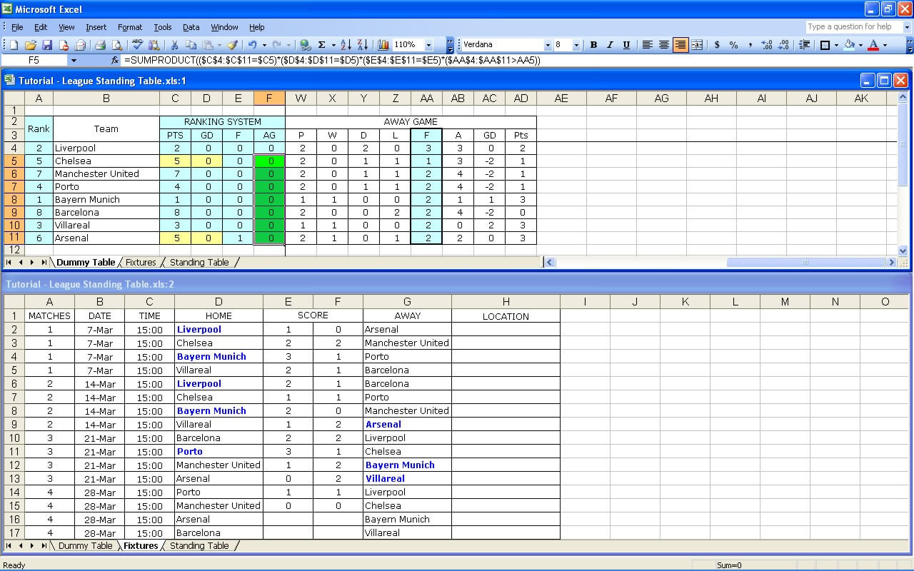
You completed your ranking table now, and what about is some teams still share the same position after competition rule number four ? You should defined additional rule and try to input it in your new columns. I think this is your homework now to solve it :-D…
If you have no problem on following my tutorial until this step, I think you are ready to expand or change the competition rules to suit your needs. Or, you can create your own sports league table.
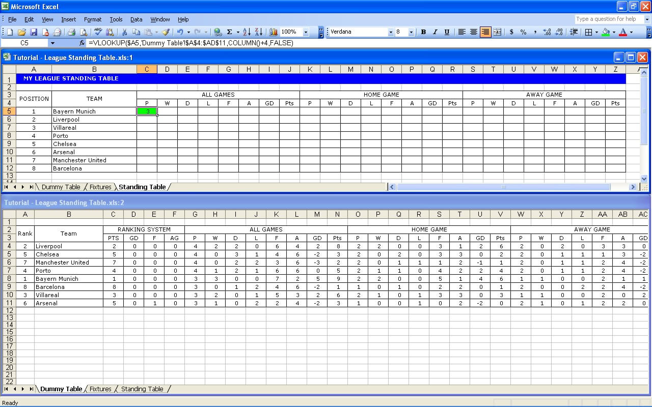
Step 22 : Create Formula to Fill Standing Table Worksheet
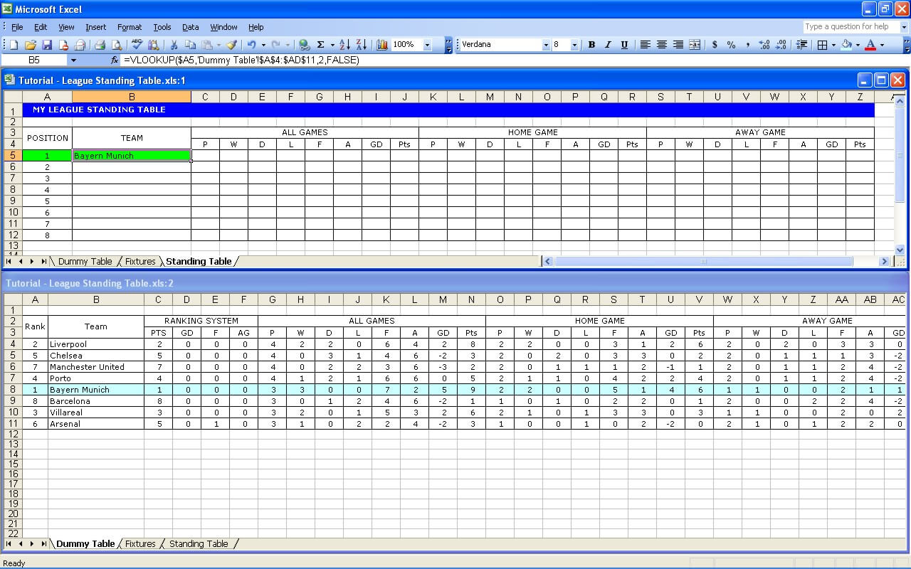
Once you finished step 19, working on this standing table worksheet is easy. All you have to do just put number 1 to 8 in position column or column A and fill all corresponding cells with the value in working sheets related with those numbers.
Let’s start creating the formula
1. Go to cell B5 and type formula Vlookup($A5,’Dummy Table’!$A$4:$AD$11,2,false)
2. Copy B5
3. Select cell B5 to B12 and paste it.
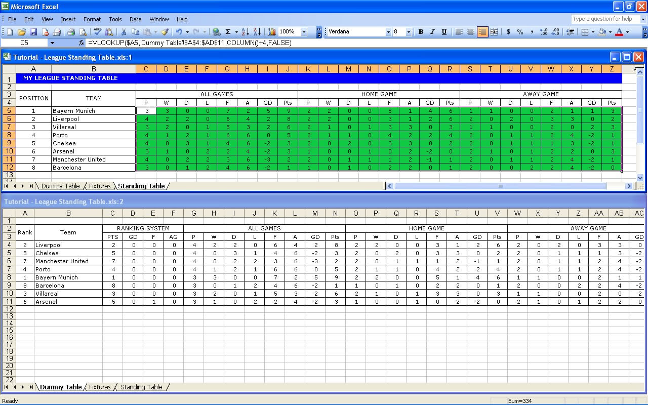
4. Select cell C5 and type formula Vlookup($A5,’Dummy Table’!$A$4:$AD$11,COLUMN()+4,false)
5. Copy C5
6. Select cell C5 – Z12 and paste it.
You have your standing table completed now.
Step 23 : Simulate Competition Full Matches
This is the last thing to do but the most important part of your work, just like when you sell a product and you do a quality test to make sure your product meets all the specification, you need to simulate the competition on your sheets by putting dummy team fixtures and points in fixtures worksheet and see the results. If you want to be more precise, you have to simulate all conditions that might happens to make sure that your formula is working well.
That’s all guys. Let me know if you have problems. I will answer it in my spare time, but, tell you the truth, do not expect me to answer it quickly.
NOTES:
Perhaps there is some mistyping in formula written in this tutorial. If you found one, please refer to the correct one in excel function box in images I attached. And please let me know so I can correct it. Thanks.
How can I create a NHL-hockey style league fixture and table?
Hi there,
just wanted to say thank you for the above – brilliant tutorial and I have achieved setting up my own league from it – even with ranking that goes down to alphabetical if not differentiated by preceding conditions!! Must be nice to know this is still helpful so many years on!! Thanks again
HI Chris could you help me with the formula for ranking to alphabetical please, would be much appreciated, I am totally stumped on this one
Gracias por toda la informacion sobre Excel.
Sería posible una plantilla para campeonatos Nacionales o Interncionales de Baloncesto.
Que diferencias podria haber con las plantillas de futbol.
Gracias.
Is there a way of offering a team an extra point if they lost by less than or equal to 50% of the score (for netball leagues)? E.g 5-3. The winning team would get 3 points for winning, the losing team would get an extra point because they scored 3 goals (less than 50% of the score).
Or a way of adding additional points to a team and I insert it manually when they lose by less than 50%?
I used your tutorial creating teams and have been very successful with it.
There was hiccups but viewing your tutorial again and looking at previous copies of your spreadsheets made me realise what would allow me to have the team standing correct; that is without the “#N/A”. I simply pumped in a reverse ranking for the teams and incorporated that as part of the last ranking. Thus eliminating all “#N/A” and having all teams shown on order of ranking.
Wonderful spreadsheet to use.
How can you add a Last 5 games tables? So win draw lose GoalsFor and GoalsAgainst?
Btw I LOVE your spreadsheet and clear explanation!!
Hi, congratulations for your wonderful job.
I’ve been using the Tennis Tournament Brackets template, and it’s been very useful; but i’ve found a little issue, because a tennis game can have a W.O result, or a desistence (give up) of one of the players, or even a third set of super tiebreak, which result can be 12 x 7, or 18 x 12, or etc, and the spreadsheet doesn’t recognize none of them. Could you fix it in a new version of it?
I’d be even more grateful.
Regards,
Artur.
Thank you thank you thank you. This was a terrific help and I really appreciate you explaining the logic behind the formulas. Cheers you and your favorite team(s).
Thank you for so much information.Getting help with Excel formulas is like pulling teeth and you have advanced me light years. Can you help me with Bonus points? I am applying your information to Super 15 Rugby. For 4 (Tries) goals scored in a match the Team receives 1 Bonus Point. If the Team loses within 7 or less points the losing Team can gain 2 Bonus Points from a game. I have tried to figure this out using what you have shown without any success. There are other formulas I need for Rugby but this will help for now. Thanking you in advance.
thanks for this… ???? can you tell me how to do head to head record betveen two teams???
would like to adapt this table for netball but dont know the formular for this rules:
4 points awarded for a win
3 points awarded for a draw
2 points awarded for a loss 50+ goaled scored (4-3)
1 point awarded for a loss 50 – goaled scored (4-2)
Its the points for goal difference that Im having problems with. Can you help?
I am confused with the Standing Table
Vlookup($A5,’Dummy Table’!$A$4:$AD$11,COLUMN()+4,false)
This is my final hurdle. Picture 38.
Regards,
Denzil
Create Sports League Standing Table how to download
Pleaseeee Create Sports League Standing Table.
Create Sports League Standing Table
Hello, Your tutorial is wonderful, but I am having serious difficulties with the last step. Please help me. Everytime I use the formula given, The standing Table uses incorrect data. Thanks in Advance!
Hi, this info proved to be very helpfull, one thing though, how do I get my hands on the Sports League Standing Table template?
Hi, we have junior club running on volunteer base. I’m trying to create a simple standing with six team without home or away. It should only show the standing results of six team with 10 matches Did anyone have the template. Could you share with me.
Great tutorial. I have managed everything, apart from managing to get all my participants in the correct position using rules. No matter what the rules are always the same and then they’re not appearing in the final table. Any idea how I can insert rule that displays the next one when there are the same position please?
Hello, i am a school student in the final year and i was just wondering if you could give me further information on the formulas and stuff seeing as the research task of our GCSE is to create a sports table including subs money fixtures and results?.. please let me know. Much thanks.
Hi, I’ve used this template with some changes to allow head-to-head rules to be applied (such as those used in La Liga in Spain etc) without using any macros (formula only).
Basically you need to use a fixture grid to calculate it. Hopefully the owner of this site will contact me and I can provide files to share with everyone?
I am trying to figure out how many widgets I need to order for every item listed. I have a sheet of items (rows) where for each row there may be a quantity needed or not. For each row that has an amount needed, I need to produce another sheet with ONLY the rows where there is an actual need with the quantity needed, item name and state. Here is sample data of the inventory in Worksheet A:
Name State Qty
Apples WA 5
Oranges FL
Car MI 8
Furniture VA 3
Corn IN
Notice that the Qty is null in many of the rows. Desired output on Worksheet B:
Name State Qty
Apples WA 5
Car MI 8
Furniture VA 3
So the output does not include the empty qty records. I’ve tried various vlookup formulas and others and am just having a hard time. I’d prefer to do this with a formula rather than macro or such and not using a filter. Any assistance would be appreciated.
First of all, I think these templates are great, amazing free resouce!
Used one for a 20 team league I ran last year but this year it reduced to 16 so am having to create my own from this tutorial.
Am using this template in Open Office. Have got to step 6 and entered the for formula into Cell L4 but it just says #Name? Not sure whether this is somethign to do with Office or not. Have double checked I have created the template of three sheets correctly to this point and I think I have. Can you help?
Thanks.
Did anyone hear back on how to do the head to head or know how to do the head to head when two or more teams are tied?
This is a great templte.
I was just wondering how do I change the rule for a win from 3 points to just 2points
Thanks In Advance
Walshey
How do I download the files?
Hello,
Thank you for this great and useful effort, which did help me a lot (also did enrich my excel knowledge) to create my own sheets, by using and understanding the formulas in your sheet.
I did start adding some simple math formulas to get some statics and information like (best scorer, best defender, most wining team least wining, most defeats ……etc)
But still I have difficulties with some formulas to define statics like, consecutive wins and defeats, biggest margins, comparing charts, links to individual team weekly results …etc.
I do appreciate your help if you have any sheet with data base table explaining the formulas I can use to do expand my statics.
Thank you again.
Hello, thankyou for this great explanation, i’m trying to make a sheet for la liga and i need a formula for the head 2 head matches once two teams are tied in the points. is there any formula or sth?
How can I hide the way of working for others
Hello. I currently have an excel spreadsheet which calculates and separates a league table of 6 teams via points, then goal difference and then goals scored. How can I improve this further by then separating teams that are still the same by the match result between the two teams??
Hope you can help. Very helpful thread! Many thanks, Scott
¡Hola!
Muchas gracias por sus enseñanzas, he tratado de hacer un fixture de españa, la competición “COPA DEL REY” usando la plantilla de Badminton Tournament Brackets V1.0 Pero no soy capaz de resolver una formula espero que me ayudes son dos partidos ida y vuelta y la diferencia de gol del visitante vale por dos o sea el equipo1 gana (2-1)y el equipo2 gana (1-0),pasa de ronda el equipo2 porque gol de visitante vale por dos espero que me audes o que lo puedas hacer el fixture.
Gracias!!!!!!!
Thank you very much for your lessons,I have spent years trying to solve this puzzle.I have followed your 4 rule and simulated the 2010/2011 English premier league,my complication is that Sunderland and Bolton are currently standing on equal grounds even after taking the 4 rule approach,it appears to me the only other next step to rank them is by alphabet,how then do we incorporate this situation.
Thank you
Hi,
First Thanks a lot for the useful tips. I Really enjoy it..
I have some problems if u could solve please:
1.What if, for example, two teams have same values on everything?I’m confused cause in my own sheet when 2 teams have this situation the table doesnt work…
2. How to have stats of every team by team like the one you made on your own sheets?
3. As you know in Spain the rules of sorting is different as it 2 teams with same points ranked by their head to head match. Any idea of how to solve it?
Hello Excel Guru,
You have some great, helpful info here. Do you have any idea how I would attack the following in a spread sheet?
Would like to have excel calculate team vs team lifetime records from data, is that possible?
Example You would select both teams and it would tell you the win/loss record between the two, and perhaps bring up the scores of those games.
Have 6 years of stats I would like to apply this to.
Thanks
How can i add a head-to-head points when teams are tied.
Hi, this is a really useful guide, is there any way to set this up with overtime results as my ice hockey competition does not have any draws if the game is tied at 60 mins, there is overtime and a shootout if necessary at the winner gets the 2 points but the loser still gets 1 point, like the NHL.
Any advice would be great.
Thanks.
Hi, I am having the same problem as saurabh (August 8th, 2009 6:24 pm). Everything was working great until the last step, it ranks the teams in the Standings Table correctly, but can’t get the games’ details (P,W,D,Pts,etc) into the Standings Table. Please help.
Hi I have been asked to run a patence competition, what I need is a template to work like this, round 1 a,b,c,d play against e,f,g,h and so for up to 48 players. round 2 to be a,f,j,x play against b,y,k,l IE no player in same team twice Scoring is up to 9, 11 or 15 depending on how many playyers and time. Ie if a wins 11 7 and loses 4 11 then he would have atotal of 15 points Help please
Regards
Jac
Sorry the pictures are 38 & 39 that are missing when i click them
I have learn loads from this, thanks
by the way, pictures 28 & 29 do not expand when you click them, i get a 404 error.
This is great! Thank You very much! How can I learn this formulas? There are so much formulas in one cell. I wish to create my league with 16 or… teams.10-4!
hi,
thanks for this info its been terrific help, but im only doing a small league of snooker teams, 10 teams so the ranking system is not sorting all my teams out into correct order, because alot of the teams are on identical points, any help on adding a ranking system formula to this to sort out into alphabetical order would be appreciated? thanks
Hi,
I’ve followed this tutorial through, and seem to have done everything right, but, when I come to do step 22 in Part 11, it doesn’t automatically sort the data. How do I set it up to do that?
Thanks.
This looks great and will be really useful. In the World Cup 1st round groups (Football/Soccer), teams that are level are split based on their head-to-head record (after points, GD and GF). If this involves 2 teams then it relies on them not having drawn their game, but if three teams are level, it needs to reflect the H2H of the three teams including GD and GF in those games only.
Can you think of a way that this can be done – it is quite a challenge I have found!
Many thanks
Have you considered something similar for the National Hockey League? Thirty teams, six divisions and 82 games each and the added complications of a shoot-out to decide a winner?
all problems are now solved
by a little bit of thinking ????
this tutorial was so useful for me
thanks a lot
Well, problem solved, i used double )) instead of one )
still having problem in sharing the ranks
I mean even if they don’t share the rank, how can I get rid of the #N/A that appears
if you need a screen shot you have my mail, I’ll try to explain more
thanks in advance
Hello again
I am facing this problem now
when I type the names of clubs in the fixtures sheet
without any score. the dummy sheet calculates a draw for the whole week
how can I solve this ?
Thanks in advance
@Bob Mcneil: The easiest way is just to put the coefficient number based on the order of alphabet of those 20 teams and put it into position calculation.
Regards
Greetings and thanks for a wonderful tutorial. I have used it to create my own EPL spreadsheet. Here is the problem I have. Say two(or three) teams are equal in points, goal difference and goals scored. Now I want to place (rank) those equal teams based on Alphabet. I have read and read many examples, but I can not figure it out.
I would appreciate any help with this issue
And again thanks for a great tutorial
hi saurabh,
could you inform me more detail information about your steps on applying the formula? Or you can email me.
regards
I have been able to follow every step till the last one. I am stuck at the last step and can’t figure out your formula for standing table worksheet. I am not been able to generate results by entering the above mentioned formula.
pls help
here,i have a 16 teams to plays a football tournament,so i want to make a knock out system.thats why i have a small problem on make a fixture
Hi Bernie,
I still trying to understand your point here. The easiest way I can suggest based on my understanding is as follows :
a. Create additional 3 tables (top-6, middle-7, bottom-7) that separated from the main table.
b. Put an equal formula for the team name in that 3 tables the same with the team name from main table based on their latest position
c. Put Milan in the bottom of each table, so the tables will consist Milan as its 7th or 8th team
d. Put comparison formula that will prevent Milan for shown twice if in those tables (you can use if condition).
e. Do the same step as in my tutorial post to find out the W/D/L condition and rank position
And you will have Milan record compared to other teams in those 3 tables.
I hope I interpreted your meaning correctly and this steps can solve your problems.
Regards
Greetings, your spreadsheets have been fantastic. There refinement puts my pages to shame. I have been working with your pages try to configure a additional table, and I though you might be able to help. What I would like to see in an additional table is a clubs W/D/L standing in relation to their opponents standing in the table. Example: Dividing the table into three catigories; top 6, middle 7, bottom 7. What is “Milan’s” W/D/L standing when they play against clubs that are at the top or middle or bottom the the table? This way I could see at a glance how each club is doing home and away against the strong, average and low quality clubs throughout a season. Do have any idea for a formula based on your spreadsheet that would quickly calculate these results in a table? Because right now I am tracking by hand which is, over a season, a lot of lengthy work. Any help you might have on a formula would be great.
Thanks
Hi Jeffry,
Thanks for your comments. My answers to your comments are as follows :
a. You can do that using conditional formatting, go to menu > format > conditional formatting. You can read in excel help how to use this function in detail and you can see the sample of the usage from my other football template.
b. I don’t recommend to have only one cell as the result cell, because it is easier to process the result if the goals are separated in different cells, like in my football template.
Regards
Hello Again
What would be the formula or tutorial to effect..
a) Change of font and cell to Bold letters when typed and change of cell background well score is entered in cell.
b) To get a score result to read and change automatically in a single cell eg 5-2, five goals for and two against. I would appreciate very much help in this.
Thanks God bless
Jeffrey
Hello
Thanks a million for this rather inspiring and informative tutorial. Often people with knowledge and expertise like you would rather take it to the grave with them than share it with those less fortunate. Thanks for teaching me “how to fish” a folklore in my country. Do continue the great work you are doing. Every good wish and God bless.
Very much appreciated
Jeffrey
I really like this way of doing things, it seems a lot cleaner than the way I was doing things.
I set up a similar spreadsheat, but I divided the goal difference by 10000 and then added it to the points and then took the rank from that. If a team had a +10000 Goal Difference in a season it would be worth a point.
It would be interesting to know about how you go about a knockout competition.
I have the last 5 games working – sorry – its just the goals part that im lacking!!!
HI Tomsyn, would you be able to share how you got the last five games working please?
I am having problem with Colum K Value in Home Games?
Cell Value = sumproduct((ConditionA)*(ConditionB)*(ConditionC)*()…)
Does not work?
It tells me to put (‘)…) This not work ether?
Can you help me.
Everything else up to now is Ok.
When i enter the formula for Draws it gives me an error because it doesnt seem to like the “” part of the formula (says the formual contains unrecognised text) i am using Excel 2016 is anyone able to advise
You are not really telling us how to define different things, for example 1. Define Participant Teams, you are only telling us to define them, but not how to do it on Excel. I don’t have that good Excel knowledge and experience so I would like to know how to define these things in the program.
Good day how do you present forthcoming soccer fixtures with log positions next to them
kind regards
The last step is not working! Can you help here…Vlookup($A5,’Dummy Table’!$A$4:$AD$11,COLUMN()+4,false)
This is a wonderful resource as I am now creating my own template for competitions I follow. I do run into an issue in Step 10 where the formula provided (although adjusted for my spreadsheet) results in an error message #NAME?. My formula is =SUMPRODUCT((FIXTURES!$C$2:$C$37=$B3)*(FIXTURES!$D$2:$D$37=FIXTURES!$F$2:$F$37)*(Fixtures!$D$2:$D$37””)). When I remove Condition C = Fixtures!D$2:D$52”” I do count the draws for either the home or away games but when I zero out all the fixture results at the start of the competition lots of errors show up in the dummy and standing tables. Any help would be welcome.
Do you have a model for rugby union under the following conditions please?
Win…. 4 points
draw 2…… points for each team
lost with 7 points and less…. 1 point
4 tries …..1 point
have you a league table download ?
Chris please help me out oooh
Really enjoying using this tutorial to create a League Table. However like someone else, I do encounter an error at about stage 10, following your example. On my doing the Drawn games, I get an error with the Team name (B4(, whatever name I put there, but it works for the Win formula. Error returns a #NAME? error, which then of course has a knock on effect for the following on calculations.
Please any help that you can give.
Hi, I would like to make excel table for ordinary tennis league, but if 2 teams are equal with points than it should take into account their mutual match, so who won the match is higher ranking.
So, I have 11 teams, namely:
Team 1
Team2
Team3
Team4
Team5
Team6
Team7
Team8
Team9
Team10
Team11
After entering the results for each round, let Excel itself sort the Teams in the following order:
a) Team with most points is highest ranking.
b) If 2 teams with the same nr. of points, head-to-head is then watched and whoever won is higher ranking. If the teams have not yet played each other or have result for draw, then skip to c).
c) If the teams are still the same, then they are judged by goal difference – higher difference is higher ranking.
d) If the teams are still the same, then see who received fewer goals – who received less goals is higher ranking..
e If the teams are still the same, then see who scored more goals – who scored more goals is higher ranking.
f) If the teams are still the same, then they occupy the same ranking place.
Here is link for demo file:
https://docs.google.com/spreadsheets/d/1MvQz0USGOsceyaHEFGpgTNRPL9hxbGGR/edit?rtpof=true&sd=true
If you have any solution / formula, pls let me know
Regards
Please can I play it
Thank you very much, it was a huge help.
I did it with only 12 teams.
However, I have a question, since in our hockey league there are different rules for the same score.
The first rule, which was also in the table here, is the most points.
However, goal percentage is the third rule, I did this by putting it in the third column.
The second rule is the results against each other.
And it doesn’t matter where the match was played.
I have no idea how to do this.
I would really appreciate your help.
group fixtures and league table tournament