17 MVP tips, tricks and shortcuts for Excel
Who doesn’t know Microsoft Excel? If for some reason you missed the last 33 years of Excel’s lifetime, the tl;dr version is that it is the premier spreadsheet program that can do it all. It is the Freddie Mercury of spreadsheet software — its range unmatched by any of its competitors. It is so well built that you hardly ever need to do anything manually… that is, if you know the right formulas, functions, shortcuts and all that jazz.
If you are an Excel beginner, and you want to give yourself a knowledge boost, here is our article on the best tools and sites to practice and learn Excel.
The issue many Excel users face is that it’s so densely packed with useful tools that even accomplished veterans get lost, and beginners get easily overwhelmed. They need a guru. A Yoda. Someone to explain to them the intricate details of the world of Excel and the dangers of the dark side of the Force. But who is knowledgeable enough to tackle this untacklable subject? Who could be their guide?
As it turns out, a number of people. Bill Gates, for one. But, in case you don’t have his number on speed dial, you could try Microsoft’s MVPs (Most Valuable Professionals). For years, Microsoft has been awarding its best-of-the-best, which is a good deal for them. But it’s a bigger deal for the rest of us.
The Excel MVPs are recognized as true VBA wizards, but instead of packing a magic wand and practicing telekinesis, they think in spreadsheets and channel their powers to save humanity. If you think we are exaggerating, we’re not.
These guys have made tremendous contributions to the community over the years, in various shapes and forms. They run forums and message boards, produce videos, write books and tutorials and are 100% passionate for spreadsheets. Nevertheless, as powerful as Excel can be to those who’ve mastered its dark arts, it can also be more frustrating than non-skippable game ads for normal people.
Luckily, the MVP’s are far from normal. Which is precisely why we reached out to 154 MVPs and asked them to share their best tips, tricks, and shortcuts. With great power comes great responsibility, and the Excel wizards of the world were more than willing to put on their superhero capes and save the day. So, let’s venture into expert wisdom territory, shall we?
Shortcuts
1. Alt + down arrow
Adam Kopeć / Excel i Adam
Currently, my favorite keyboard shortcut is Alt+Down Arrow. This allows you to create an instant drop-down list in a given cell. The list is based on data that is in the same column as the cell on which we used the keyboard shortcut. We just need to remember that the cell in which we want to use the instant drop-down list adjoins the data already entered (there was no empty data row between the data).
The Alt + down arrow combination also expands existing drop-down lists. This allows us to speed up our work if we focus on using the keyboard. It can also expand the filter menu in both standard data and pivot tables.
You can also move between elements of the chart with Alt + down arrow combination.
2. Alt-T-I and Alt-T-M-S
Ron de Bruin / Excel Automation
My Favorite shortcut for Win Excel. By pressing Alt+T, you can refer to the old menu structure that we used before Excel 2007. For example, to open the add-ins dialog to close or open add-ins you can use the shortcut Alt+T+I (the old Tools>Add-ins). If you want to open the Security dialog, you can use Alt+T+M+S (the old Tools>Macro>Security). You see that this is much easier than using File>Options>Trust Center>Trust Center Settings>Macro Settings.
You can check out how to disable it here.
3. Alt+F11 and Alt+F10
Jamie Garroch / Bright Carbon
I specialize in automating Microsoft Office applications by developing VBA macros and add-ins. I write VBA code to interface Excel with PowerPoint and vice versa. For example, it’s possible to programmatically create slides in PowerPoint from ranges and charts within Excel or, in the reverse direction, send content from a table in a PowerPoint slide to an Excel worksheet. You can learn more about VBA here.
My favorite shortcut is Alt+F11 to open the VBE (Visual Basic Editor). From a non-programming perspective, Alt+F10 would be my favorite shortcut. This opens the Selection Pane which you use to reorder and rename the layers of shapes in your worksheet.
4. Ctrl+T
Ajay Anand / XL n CAD
My favorite Excel Shortcut is Ctrl+T. It is the shortcut to Convert the data into an Excel Table.
Converting data into an Excel Table is the best way to keep your data organized. As soon as a data range is converted into an Excel Table, it will acquire a set of awesome properties which makes the data easy to handle.
Some solid reasons to use Excel Tables include:
- Excel Tables are easy to Create, are Dynamic and come with Slicers
- Excel Tables can create human-readable, meaningful formulas which will be easy to understand
- Excel Tables are powered with Calculated Columns
Bonus Tip: CTRL+L is a lesser known shortcut to convert a data range into an Excel Table.
You can learn more about Excel Tables here.
5. F9
Nikolay Pavlov / Планета Excel
Select a logically completed part of a complex nested formula and press F9. Excel will calculate (evaluate) the selected fragment and show it’s result.
This is the best technique for debugging complex and bulky formulas.
6. F4
Chris Newman / The Spreadsheet Guru
One of my favorite Excel “tricks” to share with users is the keyboard shortcut for Repeat. By using the F4 key, you can have Excel repeat your last spreadsheet action as many times as you wish.
This is great for repeating a change in fill color, deleting a selected row, or applying a custom cell border throughout your spreadsheet. I regard the F4 shortcut as the MOST powerful keyboard shortcut in Excel for the very simple reason that you can use a single key to carry out virtually any action done to your spreadsheet without having to memorize all the unique shortcut combinations.
It still baffles me that this shortcut is not broadly known/used by most Excel users. I personally spent years using Excel before I stumbled across the F4 shortcut’s alternative use outside of cycling through the dollar sign combinations in a formula’s cell reference (which is a more well-known use of the F4 key). This is a shortcut that will take some time to mentally remember it’s available to you, but once you are comfortable using it, your efficiency in Excel will begin to skyrocket!
7. Ctrl+Shift+L
Sumit Bansal / TrumpExcel.com
Since I work with a lot of data, my favorite shortcut is Control+Shift+L. This will apply the filter to the header row. Once the filter is applied, I can easily access the options to filter the data based on text or value.
Tips and Tricks
8. Learn power query
Matt Allington / Excelerator BI
My number 1 tip is, “Learn Power Query.” Power Query is a product that has been available inside Excel since July 2013 (7 years ago). Despite it now being a mature product, most people that I train and teach have never heard of it. Power Query is one of the best additions to Excel since Excel was first introduced more than 30 years ago.
Part of the reason so many people don’t know about it is that it is hidden in plain sight. In Excel 2016, you can find it on the Data Ribbon in the section “Get and Transform Data”; this IS Power Query. If you spend hours of time regularly cleaning, combing and reshaping raw data into something that you can use, then Power Query is the friend you have been missing.
Sumit Bansal from Trump Excel agrees
“As a part of my work, I often download multiple Excel files (or CSV files) and then need to combine these to get a consolidated data file. With Power Query, I can easily combine all the files in a folder (as long as the data structure of all these files is the same).
I find this immensely useful and I don’t need to open each file and copy-paste the data. This trick alone saves me hours of effort every week.”
9. Data types
Guillaume Gaudfroy / KPI Consulting
I love being able to connect my Power BI Service cubes to Excel with the “Data types” functionality.
The advantage is to be able to use them with simple functions and functions like “ValeurCube.”
10. Data validation
Liam Bastick / SumProduct
By far and away the most popular ‘trick’ (in all senses of the word!) I demonstrate in training sessions is this monster.
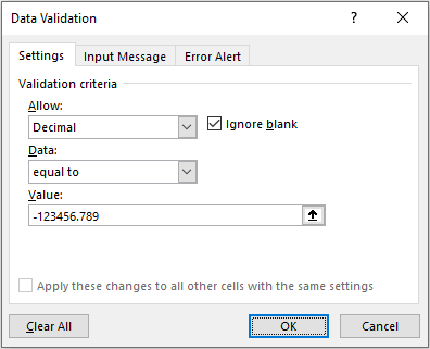
Data Validation is a useful way to control what end users can type into a worksheet cell. You can use this functionality to play a trick. Please use this at your own risk: if you get fired, you will get no sympathy here.
If someone is unfortunate enough to leave a spreadsheet unprotected, simply highlight the whole worksheet and then activate Data Validation (Data -> Data Validation -> Data Validation… or ALT+D+L). In the ‘Settings’ tab, select settings similar to the following (the aim is to pick a number the user won’t be able to guess):
Then, select the ‘Error Alert’ tab:
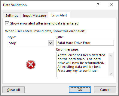
Now, de-select the range and wait for your victim to use the worksheet. As soon as they type an invalid entry, they will be greeted with the following error alert:

Who says spreadsheets can’t be fun…?
11. Coloring the active cell, its row, or its column
Tom Urtis / Atlas PM
There are two methods by which a cell can show a color: by assigning a color to its Interior property, or by Conditional Formatting. Both methods can be done manually without any programming. However, when you want a cell’s color to follow an action such as having a distinct color to the selected cell, that would require a VBA (Visual Basic for Applications) procedure called the Worksheet_SelectionChange event.
Here are 3 examples and their respective Worksheet_SelectionChange event procedures, when you change the cell’s interior color.
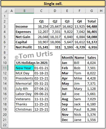
In the worksheet module for a single selected cell:
Private Sub Worksheet_SelectionChange(ByVal Target As Range)
If Target.Cells.Count > 1 Then Exit Sub
Cells.Interior.ColorIndex = 0
Target.Interior.Color = vbCyan
End Sub
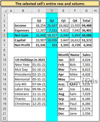
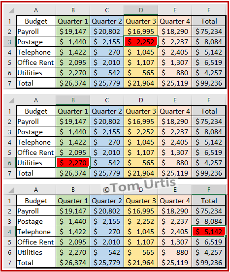
In the worksheet module for the selected cell’s entire row and column:
Private Sub Worksheet_SelectionChange(ByVal Target As Range)
If Target.Cells.Count > 1 Then Exit Sub
Cells.Interior.ColorIndex = 0
With Target
.EntireColumn.Interior.Color = vbCyan
.EntireRow.Interior.Color = vbCyan
End With
End Sub
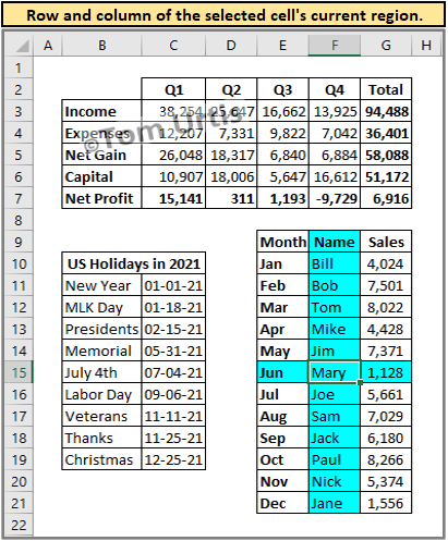
In the worksheet module for the selected cell’s current region:
Private Sub Worksheet_SelectionChange(ByVal Target As Range)
Cells.Interior.ColorIndex = 0
If IsEmpty(Target) Or Target.Cells.Count > 1 Then Exit Sub
With Target
Range(Cells(.Row, .CurrentRegion.Column), _
Cells(.Row, .CurrentRegion.Columns.Count + _
.CurrentRegion.Column – 1)).Interior.Color = vbCyan
Range(Cells(.CurrentRegion.Row, .Column), _
Cells(.CurrentRegion.Rows.Count + _
.CurrentRegion.Row – 1, .Column)).Interior.Color = vbCyan
End With
End Sub
When there are existing colors in worksheet cells that you do not want to permanently override as the previous 3 examples would do, you can use Conditional Formatting in your code, for example:
In the worksheet module for a single selected cell using Conditional Formatting:
Private Sub Worksheet_SelectionChange(ByVal Target As Range)
Cells.FormatConditions.Delete
With Target
.FormatConditions.Add xlExpression, , “TRUE”
.FormatConditions(1).Interior.Color = vbRed
End With
End Sub
These are Worksheet_SelectionChange events. To install this behavior for a worksheet, if you have not already done so, save your workbook as an Excel Macro-Enabled Workbook which will have the .xlsm extension. Then, right-click on your worksheet tab, select View Code, and paste either of these procedures (but not more than one at a time per worksheet) into the large white area that is the worksheet module. Press Alt+Q to return to the worksheet, then select a few cells to see the effects of the code.
12. Copy here as values only
Siddharth Rout / SiddharthRout.com
Siddharth kindly made a video for us. We have included it below followed by a transcript.
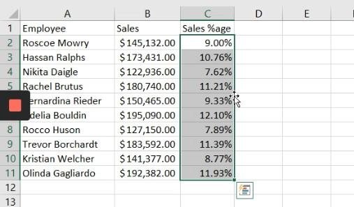
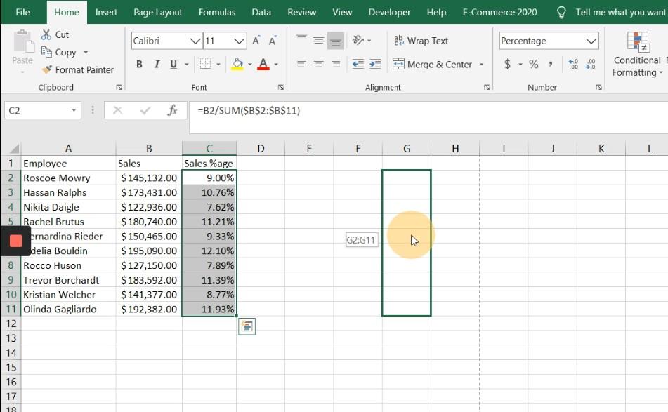
Hi, today I’m going to share an amazing Excel tip that I learned a couple of years ago. Let’s say we have this sample data:
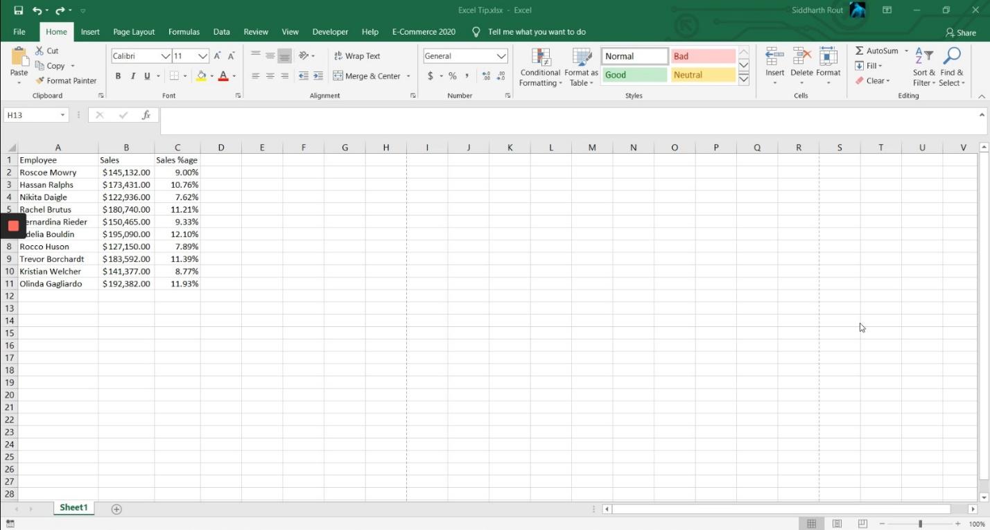
The figures are not important. The names are not important. What is important is that these cells have formulas, and I want to convert these formulas into values.
There are various ways to do it. The most conventional way and what I used to do was:
Select the range, Press Ctrl+C, right-click on it, click on 123.
Or
Right-click on the range, click on Paste Special, bring up this dialog box:
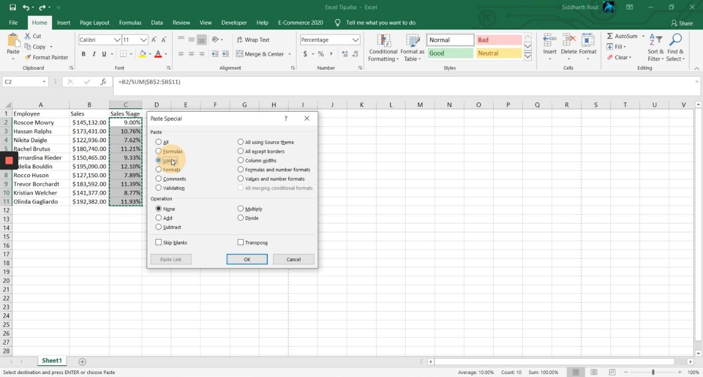
Click on Values and then click OK.
You can bring up this dialog box even from this Paste menu, which is in the Home tab by clicking on Paste Special.
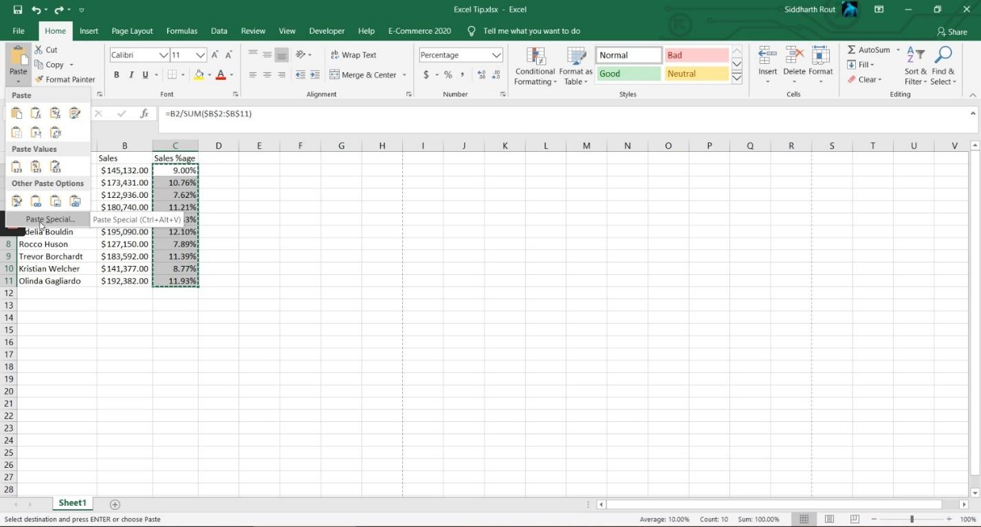
The other way is again, clicking on Paste and then clicking on 123.
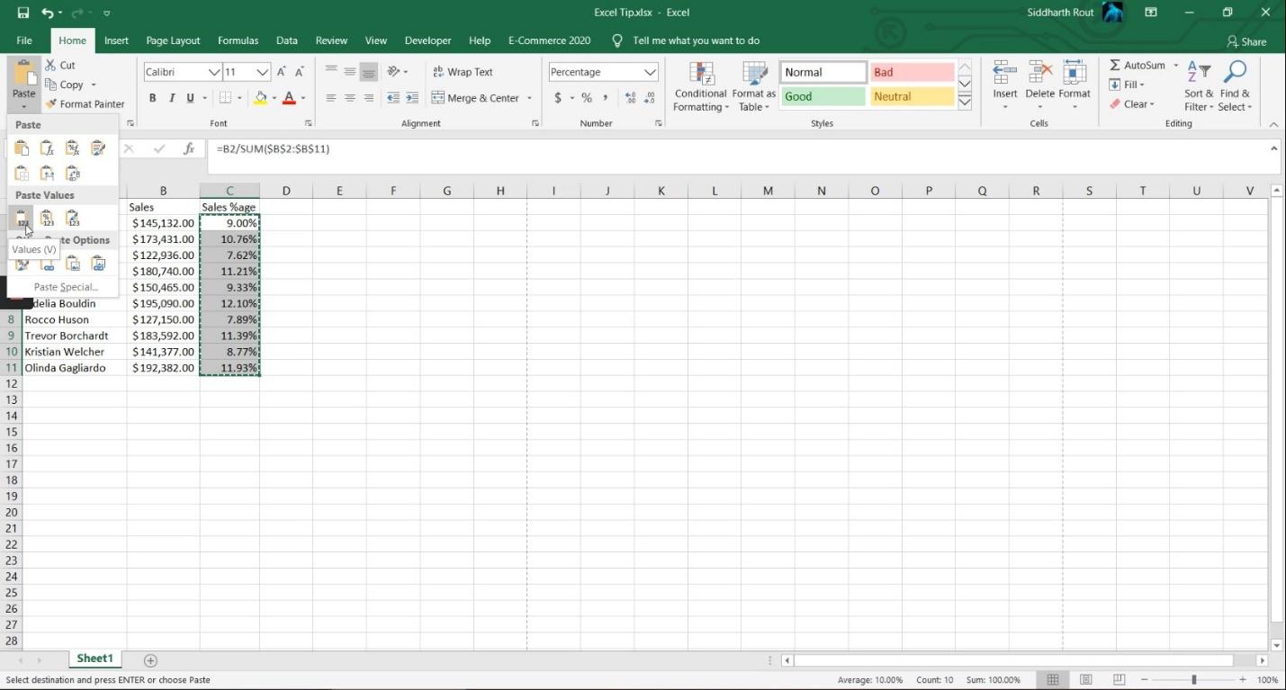
You could also bring that Paste Special dialog box by using two shortcut keys. The first is Alt+E+S, and then repeat the process.
The other shortcut key to bring this box is Ctrl+Alt+V and then select Values.
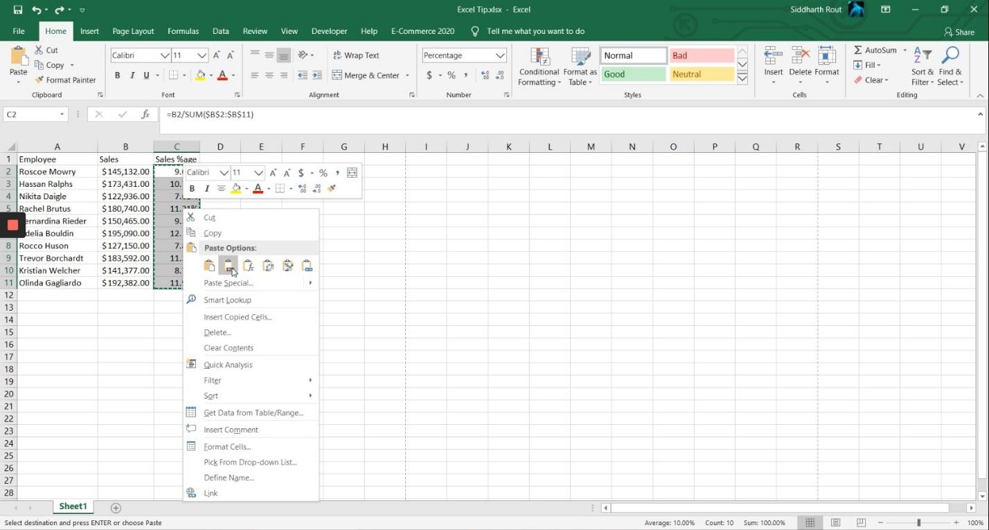
Today I’m going to share a completely different way, which does not include copying and pasting the range. What you have to do is select the range. Bring your cursor on the right border; you will see the cursor change.
Right click on it, then left click on it and drag the range to the right side:
Bring it back and then leave:
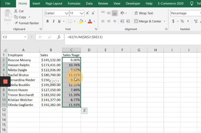
The moment you leave the mouse, you will get a menu that says Copy Here as Values Only. Simply click on it and it will convert it to values.
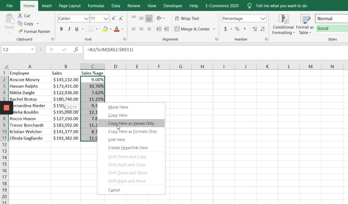
Okay, let’s do it once again: Bring the cursor on the border of the cell which has data. Right click, left click, drag to right, and then back and leave it, Copy Here as Values Only.
Isn’t this really cool?
13. A few tips and tricks
David Abiola / Excel Jet Consultant
David also made a video for us. We have included it below followed by a transcript.
In this video, we are going to see some tips and tricks. Let’s get started:
Remove Duplicates
Now, in this list, we’ll see how to remove duplicate values because we have some duplicate names. So the rule is select the data Control+Shift+Down Arrow Key, then we’ll click on the Data tab on the Data Tools group, click on Remove Duplicates, and just click on OK. So we can see seven duplicate values found and removed and we have 17 records that are unique.
Flash Fill
Now the next one, we’ll see how to do Flash Fill. In this case, we have the Full Name and we want to separate them into First Name and Last Name. Let’s first do it for the First Name. The First Name is at the leftmost (of column A) so I’m going to start by typing Laura then press Enter. The next one is Margaret. I type the first few letters, and this calls a ghost list. Click Enter. Automatically, we have names instructed. Let’s do the same thing for the Last Name, which is going to be Callahan then press Enter. Then we’ll start the other name which is Peacock, Enter. Automatically, it will fill the list as Flash Fill.
Expand/Collapse Formula Bar
The next one is how to expand and collapse the Formula Bar, if you’re writing some lengthy formula and you need to expand your formula to see all the formulas. The shortcut is Ctrl+Shift+U to expand, Ctrl+Shift+U also collapses.
Break Formula Link
Let’s see another different trick: Break Formula Link. If we look at this data, you can see we did C2 multiplied by B2 which gives us the Total. We want to break the formula to just have a single value (in the Total column). So I’m going to do Ctrl+Shift+Down Arrow Key. Then I’m going to press Ctrl+C to copy and do Alt,H,V,V, and can use the press Escape to exit out. We now have values inside the formula bar. The formula behind has been broken.
Format Painter
Now let’s go to the fourth one which is Format Painter. For the Format Painter, I’m going to just apply a color. To apply this white and this light blue, I will grab these two together. Then come to the fill color. Let’s apply this color. To apply this white and this light blue, click on Format Painter, and select these 2 rows together, press the Format Painter, and select from row #4 downwards. You can see it applies the paint.
Hide Sheet
Now let’s see another one. Occasionally, you need to hide some sheets. So you can actually hide a sheet if you just right click on the sheet to hide, and choose Hide. The sheet is hidden. To bring it back, just click on any sheet, right click and choose Unhide. Select the sheet which is hidden and click on OK, it’s back.
Format Excel Tables
The last one is how to use the Format Excel Tables. This data is in a range so to format in an Excel table, click inside the data set. Now go to the Insert tab. Under the Tables group we have the Table here, I can do Ctrl+T, and it will automatically show the Create Table dialog box. My Table’s headers have been checked automatically. Then just click OK. The formatted data is in an Excel table, and we have the Table Design contextual ribbon tab.
Hope you enjoyed this little video and if you enjoy it, stay tuned and thanks. Bye for now.
14. The UNIQUE function
Shawn Doward / lifehacks365.com
Have you ever wanted to get a list of unique values from data in your spreadsheet? ME TOO!! I love using the array function UNIQUE for just that! Combine that with the FILTER function and even more magic can happen! The UNIQUE function does not just work with your column values, it also works in rows! That’s right, get a unique list of values for the entire row, or the entire column. Don’t let UNIQUE(FILTER(XXXXX… scare you… nested functions rock, give them a shot. Want to know ‘how many’ items are unique in your list? Just wrap COUNTA around your UNIQUE argument. HOW AWESOME!
15. Named formulae
Roger Govier / technology4u.co.uk
I have always liked to use Named Formulae in my workbooks.
Many people refer to them as Named Ranges and they can be found on the Formulas tab under Name Manager

and when you click on Name Manager you see something like

However, they are not really named ranges, but they are formulae which refer to a range.
They can be just a single cell, e.g. Tax_Rate = $C$6 and C6 would contain the percentage figure that is applicable.
Or they could be static ranges such as
myData = $A$1:$M$30 but the Refers to part is a formula =$A$1:$M$30
or they can be Dynamic Ranges such as
myData =$A$1:INDEX($M$M,COUNTA($M:$M))
in which case the range will grow as more rows of data are added as the formula COUNTA returns an increasing number.
But the tip I would give anybody when creating named formulae is to start the name with an underscore. In the image above, I have _fc for first column, and _fr for first row, similarly _lr and _lc for last row and column. The great advantage this gives, is when using the formula editor to create formulae in your worksheet, as soon as you place an underscore you see the list of your named formulae when you use Formula Autocomplete

For those of you who have not seen this feature, you may need to turn it on in your copy of Excel. You will find it under File > Options > Formulas category and then under Working with formulas select Formula Autocomplete

For example, I might have some named formulae like this where I have data starting cell B2
| _fc | =MATCH(1,–NOT(ISBLANK(‘Data List’!$2:$2)),0) |
| _fr | =MATCH(1,–NOT(ISBLANK(‘Data List’!$B:$B)),0) |
| _lc | =MATCH(LOOKUP(2, 1/(LEN(‘Data List’!$2:$2)>0), ‘Data List’!$2:$2),’Data List’!$2:$2,0) |
| _lr | =MATCH(LOOKUP(2, 1/(LEN(‘Data List’!$B:$B)>0), ‘Data List’!$B:$B),’Data List’!$B:$B,0) |
| _drData | =INDEX(‘Data List’!$1:$10000,_fr,_fc) : INDEX(‘Data List’!$1:$10000,_lr,_lc) |
(_drData stands for Dynamic Range data, as opposed to _srData which I would know was a static range).
I have come across a lot of people when I have been giving seminars who do not realise that you can have formulae each side of the “:” operator to define ranges, as I have above.
Sure, in this case I could have used =’Data List’!$B$2 : INDEX(‘Data List’!$1:$10000,_lr,_lc), but even with just _lr and _lc defined, this is a much easier formula to read than
=’Data List’!$B$2 : INDEX(‘Data List’!$1:$10000, MATCH(LOOKUP(2, 1/(LEN(‘Data List’!$B:$B)>0), ‘Data List’!$B:$B),’Data List’!$B:$B,0)
,MATCH(LOOKUP(2, 1/(LEN(‘Data List’!$2:$2)>0), ‘Data List’!$2:$2),’Data List’!$2:$2,0)
)
So named formulae are a bit like using a helper column to break a formula down into more shorter parts which are easier to read, less error prone and easier to maintain. For example, if I had set up named formulae for _Amount and _Month,
_Amount =INDEX(‘Data List’!$J:$J,_fr+1):INDEX(‘Data List’!$J:$J,_lr)
_Month =INDEX(‘Data List’!$C:$C,_fr+1):INDEX(‘Data List’!$C:$C,_lr)
then with a Month entered in say C5 of a sheet I could have the formula
=SUMIFS(_Amount , _Month , C5) nice and simple, and clear to read.
Of course, now we have Tables, the need for dynamic ranges is not as great, but here again, I always name my tables starting with _tb, so again with Formula Complete it is easy to see a list of Tables within the workbook, hit Tab of the name and it goes into the formula

and then press “[” and you see a list of all the column headers to see which one you want, highlight and tab and it is entered.

But even though I use Tables a huge amount, I still use named formulae both to keep my formulae shorter and more readable, and to make the ranges I am selecting from dynamic so that they can alter according to values that I may have entered in other cells.
For example, with the new Dynamic Arrays and with Tables as the source data I use formulae like
=SUMIFS( _Data , _Row , H10# , _Col , L9#)
(I have deliberately put extra spaces in formula for readability)
So, in this formula _Data is referring to a column of a tables, according to what a user has selected, similarly, the _Row and _Col will choose different columns from the table to use a Crosstab report.
For those who have not seen Dynamic Arrays yet, the “#” sign after the cell reference tells Excel that this is a dynamic array anchor point for the array.
16. Making a duplicate copy of a sheet
Jon Acampora / excelcampus.com
Making a duplicate copy of a sheet can be a time consuming task. Especially if it’s something you do often. It typically requires several clicks through the sheet tab’s right-click menu. However, there is a faster way.
The quickest way I’ve found to make a duplicate copy of a sheet is to:
- Left-click and hold on the sheet you want to copy.
- Press and hold the Ctrl key. A plus symbol will appear in the sheet mouse icon.
- Drag the sheet to the right until the down arrow appears to the right of the sheet.
- Release the left mouse button. Then release the Ctrl key.

It sounds like a lot, but once you get the hang of it you will wonder how you ever lived without this trick. It’s much faster than right-clicking the tab and going to the Move or Copy… menu.
You can also first select multiple sheets with the Shift key, then use the same method to copy multiple sheets at the same time.
Bonus tip: This Ctrl & Drag method also works to make duplicate copies of shapes or charts. Select a shape/chart and then hold Ctrl while moving it. Release the mouse button and a copy of the object will be placed on the sheet. Release the Ctrl key after releasing the mouse button. Hold the Shift key with Ctrl to keep the shape vertically or horizontally aligned to the original.
BONUS
17. F#
Tomas Petricek / tomasp.net
Some people say that Excel is the most widely used functional programming language – and I think this is true. Excel is amazingly powerful and works well as long as your spreadsheets are relatively simple. But what to do if the computations that you are trying to write in Excel get bigger?
In this case, it’s worth looking for a programming language that is conceptually quite close to Excel, but lets you structure your computations better, edit them in a team and keep a history of your changes. In my experience, the F# programming language is a great answer in this case! In the trainings I do at fsharpWorks we regularly teach F# to people who come from an Excel background, but find their large spreadsheets hard to maintain. They often find that making the switch from Excel to a complete programming language is not nearly as hard as they thought!
Did you write these down? Or better yet, did you open up Excel 2019 (or whichever version you are using) and start practising straight away? Let us know which tips worked best for you and share your own discoveries on Excel exploration in the comments.
MALWAREBYTES says this WebSite is “dangerous”
18. Making dropdwon menu in spreadsheet
Shahriar Suhan
Create a drop-down list
1. Open a spreadsheet in Google Sheets.
2. Select the cell or cells where you want to create a drop-down list.
3. Click Data. …
4. Next to “Criteria,” choose an option: …
5. The cells will have a Down arrow. …
If you enter data in a cell that doesn’t match an item on the list, you’ll see a warning. …
Click Save.
Wow! No comments on such an illustrative article?
Well, not having yet read but a few (5) of the tips, I can already say that it is very useful, for 3 of those I can put to good use, and from reading the ToC I can see that there are a few others that will enlighten me to some degree. Thank you so very much for such a great compilation of tips and shortcuts.
Happy New Year and may 2021 bring you and all of us better “circumstances” than 2020 did.
Be safe and be well.
Cheers
I strongly suggest you also visit the programming notation/language: APL. It was written as a mathematical notation and then implemented on computers (mainframes and PCs). It is an array processor with great efficiency. Worth a look if you like F#.
Thank you for posting this excellent compilation. It’s both comforting and satisfying to see quite a few of the names of MVPs who were so important to me when I was just starting out in the nineties after having worked in Lotus 1-2-3 and Symphony, then Borland Quattro Pro.
There have been countless times when I have felt blessed to be standing on your shoulders!
really fascinating, excellent work and many thanks for sharing such an excellent blog These excel presentations help a lot of people who work in the corporate world.